Bayesian Generalized linear mixed models with data missing not at - PowerPoint PPT Presentation
Bayesian Generalized linear mixed models with data missing not at random Overview: Two simple introductory examples of data missing not at random (MNAR) Missing mechanism and likelihood in the case of missing at random (MAR) as defined by
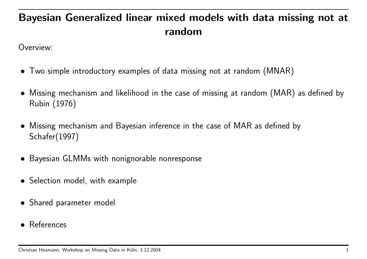
Bayesian Generalized linear mixed models with data missing not at random Overview: • Two simple introductory examples of data missing not at random (MNAR) • Missing mechanism and likelihood in the case of missing at random (MAR) as defined by Rubin (1976) • Missing mechanism and Bayesian inference in the case of MAR as defined by Schafer(1997) • Bayesian GLMMs with nonignorable nonresponse • Selection model, with example • Shared parameter model • References Christian Heumann, Workshop on Missing Data in K¨ oln, 3.12.2004 1
Random sample from a Bernoulli distribution with missing data • Let ( y 1 , . . . , y n ) an iid sample from a Bernoulli ( p ) • p = E( y i ) = P ( y i = 1) , 0 < p < 1 • m < n observations are missing: y i r i 1 1 0 1 . . . . . . 1 1 ? 0 ? 0 . . . . . . ? 0 • We introduce indicator variables r i : � 1 if y i is observed (reported) r i = 0 if y i is missing (not reported) Christian Heumann, Workshop on Missing Data in K¨ oln, 3.12.2004 2
• The indicator variables r i are also random variables • The missing process can be characterised through the conditional distributions of r i given y i : P ( r i = 1 | y i = 1) = α 1 P ( r i = 1 | y i = 0) = α 0 P ( r i = 0 | y i = 1) = 1 − α 1 P ( r i = 0 | y i = 0) = 1 − α 0 with 0 < α 0 , α 1 < 1 . • Theorem of Bayes: pα 1 E( y i | r i = 1) = P ( y i = 1 | r i = 1) = (1) pα 1 + (1 − p ) α 0 and p (1 − α 1 ) E( y i | r i = 0) = P ( y i = 1 | r i = 0) = (2) p (1 − α 1 ) + (1 − p )(1 − α 0 ) The conditional expectations in (1) und (2) are equal iff α 0 = α 1 . Christian Heumann, Workshop on Missing Data in K¨ oln, 3.12.2004 3
• On the other hand E( y i ) = p = E( y i | r i = 1) P ( r i = 1) + E( y i | r i = 0)[1 − P ( r i = 1)] (3) • The interesting question from a statistical point of view is: Can we estimate the probability or expectation p from the n − m observed values? Answer: Only if E( y i | r i = 1) = E( y i | r i = 0) in (3), that is when α 0 = α 1 holds, since then: p = E( y i | r i = 1) − → Missing (completely) at random M(C)AR • What happens if α 0 � = α 1 ? We can only estimate – E( y i | r i = 1) – P ( r i = 1) by relative frequencies. But E( y i | r i = 0) is not identifiable from the observed data − → MNAR Example: p = 0 . 4 , α 0 = 0 . 5 , α 1 = 0 . 9 . Then E( y i | r i = 1) = 0 . 55 > p − → ( � n − m i =1 y i ) / ( n − m ) (observed data) overestimates p Christian Heumann, Workshop on Missing Data in K¨ oln, 3.12.2004 4
Motivation for three different approaches to the problem of MNAR data 1. We can make some vague assumption ( − → Bayes) for α 0 und α 1 − → include missing data process in the estimation procedure for p 2. We assume P ( y i | r i = 0) = P ( y i | r i = 1) . Therefore we equate or constrain the unidentifiable parameter to an identifiable parameter. This is essentially the idea of pattern mixture models. Verbeke and Molenberghs (2000) gives an extensive and excellent overview about pattern mixture models in the context of linear mixed models and provides many references. 3. No such assumption is possible − → Compute bounds for p With (3) we have p min = E( y i | r i = 1) P ( r i = 1) < p < E( y i | r i = 1) P ( r i = 1) + [1 − P ( r i = 1)] = p max � �� � � �� � if E( y i | r i = 0) = 0 if E( y i | r i = 0) = 1 Example continued: Using the concrete numbers and (3) we get p min = 0 . 36 < p < 0 . 36 + 0 . 34 = 0 . 7 = p max Christian Heumann, Workshop on Missing Data in K¨ oln, 3.12.2004 5
This results in two sources of uncertainty for estimating p : • Uncertainty induced by the missing data through parameters which cannot be identified from the observed data • Statistical uncertainty (variance) from the estimation procedure This idea has been applied to more complex models (missing response and/or covariate data) e.g. by • Horowitz and Manski (2000) • Horowitz and Manski (2001) • Vansteelandt and Goetghebeur (2001) • Manski (2003) • Heumann(2003), Habilitation, Chapter 5 Christian Heumann, Workshop on Missing Data in K¨ oln, 3.12.2004 6
Random sample from a normal distribution with missing data • y ∼ N (0 , 1) • Missing data process is parameterised with a logistic regression model: log ( P ( r i = 1 | y i ) /P ( r i = 0 | y i )) = β 0 + β 1 y i , β 0 , β 1 ∈ R exp( β 0 + β 1 y i ) P ( r i = 1 | y i ) = 1 + exp( β 0 + β 1 y i ) • The situation is a variant of the sample selection model (Heckman, 1976), where we use the logit link instead of the probit link • If the model is correctly specified (assumption of a normal distribution is correct and the missing data process is correctly specified by the logistic model) − → Maximum Likelihood estimation is possible • Example: β 0 = − 0 . 5 , β 1 = 2 . 0 Christian Heumann, Workshop on Missing Data in K¨ oln, 3.12.2004 7
Effect of a selection model on normal data P(R=1|y)=exp(−0.5+2*y)/( 1+exp(−0.5+2*y) ) 0.5 Density of N(0,1) Kernel density estimate complete data 0.4 Kernel density estimate observed data 0.3 Density 0.2 0.1 0.0 −2 0 2 4 Christian Heumann, Workshop on Missing Data in K¨ oln, 3.12.2004 8
Asymmetric treatment of missing data in regression models • Missing response data or missing covariate data or both? • Makes a big difference! Why? • A regression model only specifies f ( y | x ; θ ) while the marginal distribution of the covariates is unspecified • One possibility for MNAR response : provide a model for the missing data process P ( r y | y, x ; ψ ) and use the selection model f ( y, r y | x ; θ, ψ ) = P ( r y | y, x ; ξ ) f ( y | x ; θ ) This has been used e.g. by Verbeke and Molenberghs (2000) for linear mixed models (LMMs) • If covariates x are MNAR then estimating a regression model conditional on x is out-of-the-box possible if we use only the complete cases (CC analysis). One possible Christian Heumann, Workshop on Missing Data in K¨ oln, 3.12.2004 9
method is to model the joint distribution of y and x instead of the conditional distribution of y given x : f ( y, x, r x | θ, ψ, ξ ) = P ( r x | y, x ; ξ ) f ( y | x ; θ ) f ( x | ψ ) This has been used by Ibrahim, Lipsitz and Chen (1999) for Generalised Linear Models (GLMs) • An interesting special case is if P ( r x | y, x ; ξ ) = P ( r x | x ; ξ ) . Then f ( y | x, r x ) = f ( y | x ) (4) – A complete case analyses (CC) which indeed models f ( y | x, r x = 1) gives a consistent estimate for θ . Christian Heumann, Workshop on Missing Data in K¨ oln, 3.12.2004 10
Characterising the missing mechanism as introduced by Rubin (1976), Little and Rubin (1987) in the context of likelihood estimation • Simplification: No distinction between response and covariates • Split data y into the two parts y = ( y obs , y mis ) • Likelihood f ( y | θ ) • Missing mechanism P ( r | y ; ξ ) = P ( r | y obs , y mis ; ξ ) • Assumption: θ ∈ Θ , ξ ∈ Ξ − → ( θ, ξ ) ∈ Θ × Ξ . θ and ξ are said to be distinct. • The expression f ( r, y | θ, ξ ) = f ( y obs , y mis | θ ) P ( r | y obs , y mis ; ξ ) is called likelihood of the complete data (or complete data likelihood ) Christian Heumann, Workshop on Missing Data in K¨ oln, 3.12.2004 11
• The expression � f ( r, y obs | θ, ξ ) = f ( y obs , y mis | θ ) P ( r | y obs , y mis ; ξ ) dy mis is called likelihood of the observed data (or observed data likelihood ) • The missing mechanism is called missing at random (MAR), if P ( r | y obs , y mis ; ξ ) = P ( r | y obs ; ξ ) does not depend on y mis . • Then: � f ( r, y obs | θ, ξ ) = f ( y obs , y mis | θ ) P ( r | y obs ; ξ ) dy mis = f ( y obs | θ ) P ( r | y obs ; ξ ) If we are only interested in inference about the parameter θ and under the assumption that θ and ξ are distinct, inference can then be based on f ( y obs | θ ) alone and the mechanism P ( r | y obs ; ξ ) can be ignored. The mechanism is then called ignorable. Christian Heumann, Workshop on Missing Data in K¨ oln, 3.12.2004 12
Extension to Bayesian inference as introduced by Schafer (1997) • Assumption of independent priors on θ und ξ : π ( θ, ξ ) = π ( θ ) π ( ξ ) • Posterior distribution: π ( θ, ξ | y obs , r ) ∝ f ( y obs , r | θ, ξ ) π ( θ ) π ( ξ ) If MAR holds: π ( θ, ξ | y obs , r ) ∝ f ( y obs | θ ) P ( r | y obs ; ξ ) π ( θ ) π ( ξ ) It follows: π ( θ | y obs ) ∝ f ( y obs | θ ) π ( θ ) Christian Heumann, Workshop on Missing Data in K¨ oln, 3.12.2004 13
• Often f ( y obs | θ ) is complicated compared to f ( y obs , y mis | θ ) . Solution through Monte Carlo techniques, e.g. data augmentation (Tanner, 1991). For s = 1 , . . . , S : – Imputation step (I–step): draw from the conditional predictive distribution y ( s ) mis ∼ f ( y mis | y obs , θ ( s ) ) – Probability step (P–step) θ ( s +1) ∼ π ( θ | y obs , y ( s ) mis ) ∝ f ( y obs , y ( s ) mis | θ ) π ( θ ) • If S is big enough, the sequences { θ ( s ) } und { y ( s ) mis } (after some burn-in) are draws from the distribution π ( θ | y obs ) and the unconditional predictive distribution f ( y mis | y obs ) − → proper imputations Christian Heumann, Workshop on Missing Data in K¨ oln, 3.12.2004 14
Recommend
More recommend
Explore More Topics
Stay informed with curated content and fresh updates.
