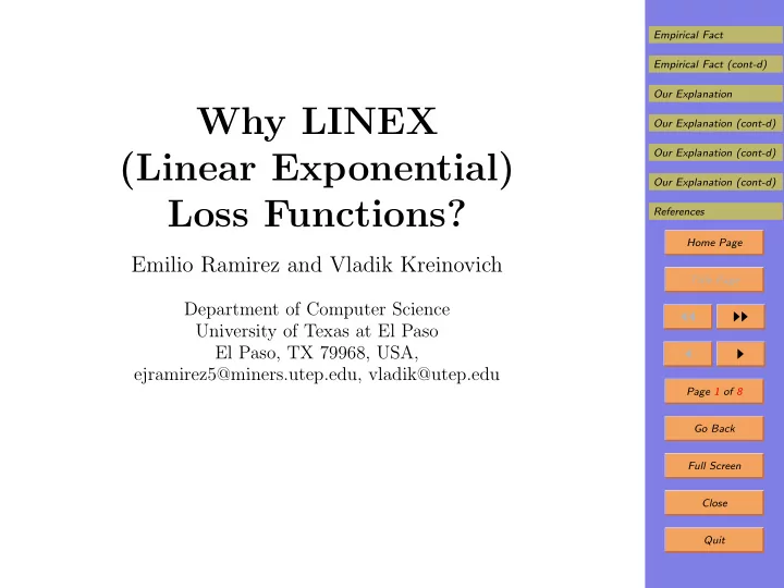
Why LINEX Our Explanation (cont-d) Our Explanation (cont-d) - PowerPoint PPT Presentation
Empirical Fact Empirical Fact (cont-d) Our Explanation Why LINEX Our Explanation (cont-d) Our Explanation (cont-d) (Linear Exponential) Our Explanation (cont-d) Loss Functions? References Home Page Emilio Ramirez and Vladik Kreinovich
Empirical Fact Empirical Fact (cont-d) Our Explanation Why LINEX Our Explanation (cont-d) Our Explanation (cont-d) (Linear Exponential) Our Explanation (cont-d) Loss Functions? References Home Page Emilio Ramirez and Vladik Kreinovich Title Page Department of Computer Science ◭◭ ◮◮ University of Texas at El Paso El Paso, TX 79968, USA, ◭ ◮ ejramirez5@miners.utep.edu, vladik@utep.edu Page 1 of 8 Go Back Full Screen Close Quit
Empirical Fact 1. Empirical Fact Empirical Fact (cont-d) • In design and control, we want to select the values of Our Explanation the parameters that minimize the losses. Our Explanation (cont-d) Our Explanation (cont-d) • Traditionally, the dependence of loss on the parameter Our Explanation (cont-d) is described by a quadratic function. References • However, for this function: Home Page – positive and negative deviations from the optimal Title Page value ◭◭ ◮◮ – lead to the exact same increase in loss. ◭ ◮ • In practice, the effects are often different. Page 2 of 8 • E.g., for a refrigerator, a decrease in temperature is Go Back rarely harmful, while an increase can spoil the food. Full Screen Close Quit
Empirical Fact 2. Empirical Fact (cont-d) Empirical Fact (cont-d) Our Explanation • It turns out that in many practical situations, Our Explanation (cont-d) – in the next approximation, Our Explanation (cont-d) – the best “asymmetric” loss function is a linear com- Our Explanation (cont-d) bination of a linear and exponential functions: References L ( x ) = c · exp( a · x ) − b · x + a 0 . Home Page Title Page • This combination is known as LINEX . ◭◭ ◮◮ • How can we explain this empirical fact? ◭ ◮ Page 3 of 8 Go Back Full Screen Close Quit
Empirical Fact 3. Our Explanation Empirical Fact (cont-d) • Quadratic functions are linear combinations of smooth Our Explanation functions 1, x , and x 2 . Our Explanation (cont-d) Our Explanation (cont-d) • The class of such functions does not change if we change Our Explanation (cont-d) the starting point for measuring x . References • Then, we replace x with x + x 0 for some x 0 . Home Page • Let us thus look for similarly “shift-invariant” smooth Title Page families of the type ◭◭ ◮◮ c 1 · f 1 ( x ) + c 2 · f 2 ( x ) + c 3 · f 3 ( x ) . ◭ ◮ • Shift-invariance means, in particular, that all shifted Page 4 of 8 functions f i ( x + x 0 ) belong to the same family. Go Back • In particular, this means that, for some value c ij ( x 0 ), we have Full Screen � f i ( x + x 0 ) = c ij ( x 0 ) · f j ( x ) . Close j Quit
Empirical Fact 4. Our Explanation (cont-d) Empirical Fact (cont-d) Our Explanation • For each i and x 0 , let us select three different values x k . Our Explanation (cont-d) • Then, we get a linear system for three unknowns c ij ( x 0 ), Our Explanation (cont-d) j = 1 , 2 , 3: Our Explanation (cont-d) � f i ( x k + x 0 ) = c ij ( x 0 ) · f j ( x k ) . References j Home Page • By Cramer’s rule, the values c ij ( x 0 ) are rational func- Title Page tions of values f i ( x k + x 0 ) and f j ( x k ). ◭◭ ◮◮ • These values smoothly depend on x 0 . ◭ ◮ • Thus, the functions c ij ( x 0 ) are also differentiable. Page 5 of 8 • So, we can differentiate the above equality with respect Go Back to x 0 . Full Screen • After the differentiation, we can take x 0 = 0 and get Close i ( x ) = � a ij · f j ( x ), where a ij def f ′ = c ′ ij (0). Quit
Empirical Fact 5. Our Explanation (cont-d) Empirical Fact (cont-d) Our Explanation • Solutions to such linear differential equations with con- stant coefficients are well known. Our Explanation (cont-d) Our Explanation (cont-d) • These solutions are linear combinations of terms Our Explanation (cont-d) x k · exp( λ · x ), where: References • λ is an eigenvalue of the matrix c ij , and Home Page • k = 0 , 1 , 2 , . . . ; k > 0 corresponds to the case of Title Page equal eigenvalues. ◭◭ ◮◮ • Quadratic functions correspond to the case when all ◭ ◮ three eigenvalues are equal to 0. Page 6 of 8 • The simplest modification is when: Go Back • one of the eigenvalues becomes different from 0, Full Screen while Close • the other two remain 0s. Quit
Empirical Fact 6. Our Explanation (cont-d) Empirical Fact (cont-d) Our Explanation • Reminder: The simplest modification is when: Our Explanation (cont-d) • one of the eigenvalues becomes different from 0, Our Explanation (cont-d) while Our Explanation (cont-d) • the other two remain 0s. References • This corresponds to the loss functions Home Page Title Page c 1 · exp( λ · x ) + c 2 · x + c 2 . ◭◭ ◮◮ • This is exactly LINEX. ◭ ◮ • Thus, the practical efficiency of LINEX loss functions Page 7 of 8 can be naturally explained. Go Back Full Screen Close Quit
7. References Empirical Fact Empirical Fact (cont-d) • Yen-Chang Chang and Wen-Liang Hung, “LINEX loss Our Explanation Our Explanation (cont-d) functions with applications to determining the opti- Our Explanation (cont-d) mum process parameters”, Quality & Quantity , 2007, Our Explanation (cont-d) Vol. 41, pp. 291–301. References • H. R. Varian, “A Bayesian approach to real estate as- Home Page sessment”, In: S. E. Fienberg and A. Zellner (eds.), Title Page Studies in Bayesian Econometrics and Statistics in Honor of Leonard L. Savage , Noth Holland, Amsterdam, 1975, ◭◭ ◮◮ 1975, pp. 195–208. ◭ ◮ • A. Zellner, “Bayesian estimation and prediction using Page 8 of 8 asymmetric loss functions”, Journal of the American Go Back Statistical Association , 1986, Vol. 81, pp. 446–451. Full Screen Close Quit
Recommend
More recommend
Explore More Topics
Stay informed with curated content and fresh updates.


