Missing Data and Imputation NINA ORWITZ OCTOBER 30 TH , 2017 - PowerPoint PPT Presentation

Missing Data and Imputation NINA ORWITZ OCTOBER 30 TH , 2017

Outline  Types of missing data  Simple methods for dealing with missing data  Single and multiple imputation  R example

Missing data is a complex problem We must consider: - The type of missingness present in our data - How different methods yield biased and/or inefficient estimates - No method perfectly “fixes” the problem of missing data

Missing Completely at Random (MCAR) If Missing= missing indicator (1=missing, 0= not missing): Pr (Missing | Xmiss, Xobs) = Pr (Missing) - Being missing is independent of both observed and unobserved data - Pr (missingness) is the same for all units - R package: Little’s MCAR test - Example: participant flips coin to decide whether to answer survey question

Missing at Random (MAR) If Missing= missing indicator (1=missing, 0= not missing): Pr (Missing | Xmiss, Xobs) = Pr (Missing | Xobs) - Pr (missingness) depends only on available information - Example: In a survey, poor subjects were less likely to answer a survey question on drug use than wealthier subjects. The missingness of drug use is related to observed predictors (income) but not drug use itself. - Problem with assuming MAR?

Missing Not at Random (MNAR) If Missing= missing indicator (1=missing, 0= not missing): Pr (Missing | Xmiss, Xobs) = Pr (Missing | Xmiss, Xobs) -Pr (missingness) depends on unobserved information, biases the model - Example 1: Suppose answering the question (from last slide) also depends on drug use itself; those who used drugs are less likely to report it. - Example 2: Those who are high earners are less likely to report their incomes.

Taking Action On Missingness - Not always necessary! - If we have ~5% missingness in a variable, estimates will not change much, probably will not be biased - If we have ~30% missingness in a variable, estimates will change a lot  reason to consider imputation methods

Complete-Case Analysis - “Listwise Deletion” - Exclude all data for a case that has 1 or more missing values - Done automatically in R for linear regression, other regressions - Assumes MCAR, biased estimates, ignoring information - Inverse Probability Weighting- used to correct for bias from this  Complete cases are weighted as the inverse of their probability of being a complete case; corrects for unequal sampling fractions

Available-Case Analysis - “Pairwise Deletion” - Can use ‘regtools’ package in R - Involves computation of pairs of variables, can include in the calculation any observations for which the pair is intact Ex: predicting weight from height, age: can estimate covariance between height and weight using all records when height and weight are intact, even if age is missing - Assumes MCAR, standard errors over or under estimated

Types of Imputation A. Single Imputation - Can take on many forms: impute the missing values based on values of other variable(s) B. Multiple Imputation - Introduced by Rubin in 1987 - Impute the missing values multiple times based on values of other variables

Single Imputation Methods Mean Imputation - Impute with the mean of the observed values of that variable. Underestimates SEs, pulls estimates of correlation toward 0 Random Imputation - replace NA’s with random sample of non - missing values from that variable LOCF (Last Observation Carried Forward) - in studies where we have “pre - treatment” and “post - treatment” measures. Conservative?

Single Imputation Methods (II) Indicator Variables for Missingness in Categorical Predictors - add an extra category that indicates missingness (if unordered categories) Regression Imputation - use models of the non-missing data to predict values of the missing data, may inflate correlation, produced biased estimates/SEs

Imputation in Genomics - Inference of unobserved genotypes done by using known haplotypes in the population - Bayesian PCA, KNN Impute, SVD Impute useful for -omics data - Some useful software packages: MaCH, Minimac, IMPUTE2, Beagle

Multiple Imputation Overview • Displaying missing data patterns • Identifying structural problems in the data and preprocessing Step 1: • Specifying conditional models Setup • Performing iterative imputation based on the conditional models • Checking fit of conditional models, seeing if imputations are reasonable Step 2: • Checking convergence of the procedure Imputation • Obtaining the completed data • Pooling the complete case analysis on imputed datasets Step 3: Analysis

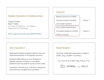
Multiple Imputation Background - Iteratively draw imputed values from the conditional distribution for each variable given the observed and imputed values of the other variables in the dataset -Markov Chain Monte Carlo Method (MCMC) assuming multivariate normality is used by default in ‘mi’ package in R  Markov Chain: sequence of R.V.s, each element’s distribution depends on value of previous element, has transitional probability, converges to stationary distribution  Monte Carlo: sampling techniques that draw pseudo-random numbers from probability distributions - Some useful R packages: MI, MICE

MCMC Method Step-By-Step 1) Replace all missing data values (X un ) with starting values 2) Estimate parameters θ from f( θ |X obs , X un ) now that we have X un from (1). 3) The next sample of X un can be drawn from Bayesian predictive distribution f(X un |X obs , θ t ) where θ t is current estimated parameter values - known as Imputation-Step (I-Step) 4) Simulate next iteration of θ from the complete data posterior distribution- -known as Prediction Step (P-Step) 5) Repeat Steps 3) and 4) iteratively until θ converges. *We can choose how many iterations we want to run in R.

Last Steps of Multiple Imputation - For each variable in the order specified, a univariate (single dependent variable) model is fit against all the predictors, and for each variable the MCMC method continues for the maximum number of iterations which allows distribution to stabilize - Check convergence of the procedure - Can increase maximum number of iterations if does not converge - Combine inferences across datasets using Rubin’s Rule

Combining Results for Inference - After imputing M datasets, final Beta estimate is mean of all of the Beta estimates from each dataset= 𝟐 𝑵 𝜸 (𝒌) 𝑵 𝒌=𝟐 𝜸 = - Total variance= variance within imputations ( A ) + variance between imputations ( B ) 𝑁 ( 1 σ 2(𝑘) + 1 + 1 1 β 𝑘 − 𝟐 𝑁 β) 2 ) = A + (1+ 𝑁 𝑘=1 𝑁−1 𝑘=1 𝑊 𝑁 ( β = 𝑵 )B 𝑁 ( 1 σ 2(𝑘) and B= ( 1 β 𝑘 − 𝑁 β) 2 ) 𝑁 𝑘=1 𝑁−1 𝑘=1 where A=

R Example NlsyV data- Subset of data on children and their families in the U.S. Outcome of interest: pprvt.36- Peabody Picture Vocabulary test score administered at 36 months Predictors: first- indicator of child being first-born or not; b.marr- indicator of mother being married when child was born; income- family income in year after child was born; momage- age of mother when child was born; momed- educational status of mother when child was born; momrace- race of mother

Drawbacks of Multiple Imputation 1. Not a perfect method- making guesses about potentially many values 2. Operates under the big assumption that all missing data is MAR 3. How many variables to include? - Too few variables increases risk of separation  when outcome is perfectly predicted by a predictor/linear combination of predictors 4. How many chains to run? Literature varies, but probably at least 5 - Can calculate based on largest proportion of missingness in a variable

Final Thoughts - There are many ways to go about imputation beyond those discussed today; increase in -omics data demands new missing data methods - Important to remember that no imputation method is perfect

References Chibnik, L. (2016). Biostatistics Workshop: Missing Data. Available from: https://www.slideshare.net/HopkinsCFAR/biostatistics-workshop-missing-data Gelman, A., & Hill, J. (2006). Missing-data imputation In Data Analysis Using Regression and Multilevel/Hierarchical Models. (Analytical Methods for Social Research, pp. 529- 544). Cambridge: Cambridge University Press. doi:10.1017/CBO9780511790942.031 Goodrich B. & Kropko, J. (2014). An Example of mi Usage. https://cran.r- project.org/web/packages/mi/vignettes/mi_vignette.pdf Schunk, D. (2008). A Markov chain Monte Carlo algorithm for multiple imputation from large surveys. A Stat. Assoc, 92, 101-114. Su, Y-S., Gelman A., Hill, J., & Yajima, M. (2011). Multiple Imputation with Diagnostics (mi) in R: Opening Windows into the Black Box. J of Stat Software, 45 (2), 1-31.