Discrete-time ChenFliess Series for Learning and Adaptive Control - PowerPoint PPT Presentation
Discrete-time ChenFliess Series for Learning and Adaptive Control W. Steven Gray Old Dominion University, Norfolk, Virginia USA ACPMS Seminar August 21, 2020 Joint work with Luis A. Duffaut Espinosa and G. S. Venkatesh . Supported by
Discrete-time Chen–Fliess Series for Learning and Adaptive Control ∗ W. Steven Gray Old Dominion University, Norfolk, Virginia USA ACPMS Seminar August 21, 2020 ∗ Joint work with Luis A. Duffaut Espinosa and G. S. Venkatesh . Supported by NSF grants CMMI-1839378 and CMMI-1839387.
ACPMS Seminar Overview 1. Motivation - The canonical control problem 2. Chen series and Chen–Fliess series 3. Discrete-time analogues 4. Implementation of a learning unit 5. Application to adaptive control 2
ACPMS Seminar 1. Motivation - The canonical control problem y u F � plant Fig. 1.1: Open-loop control • Suppose F is an operator mapping a set of input functions U to a set of output functions Y . • Select some desired y d ∈ Range( F ) ⊆ Y . • The canonical control problem is to determine a right inverse u = F − 1 [ y d ] ∈ U such that F [ u ] = ( F ◦ F − 1 )[ y d ] = y d . • Whenever F − 1 can be computed explicitly, this is called open-loop control. 3
ACPMS Seminar • In many applications F is known to be realized by some finite dimensional state space model m � z = g 0 ( z ) + ˙ g i ( z ) u i , z (0) = z 0 i =1 y j = h j ( z ) , j = 1 , . . . , ℓ, where the g i are vector fields in local coordinates, and h j maps the state to the j -th output. • If ( g, h, z 0 ) are known, then under certain conditions (well defined relative degree), F − 1 exists on a neighborhood of z 0 and is computable. • But normally a state space model is only known approximately, so this option is not always feasible. 4
ACPMS Seminar u e y d y H � F � + _ controller plant Fig. 1.2: Closed-loop control • A more practical approach is to design a mapping H : Y → U so that lim t → ∞ | y d ( t ) − y ( t ) | = 0. • This is closed-loop control via dynamic inversion. • In general closed-loop control is known to reduce the sensitivity of the output to the plant, ∂y/∂F . • The design of H still relies on some knowledge of F , usually a nominal state space model ( g, h, z 0 ). 5
ACPMS Seminar u e y d y H � F � + _ plant adaptive � controller learning unit Fig. 1.3: Adaptive closed-loop control • When F is unknown, the idea is to learn F as the system operates and then tune H in real-time. This is known as adaptive control. • All such control systems are implemented in discrete-time. • The goal is to describe an adaptive control system whose implementation utilizes a discrete-time Chen–Fliess series. 6
ACPMS Seminar 2. Chen series and Chen–Fliess series Definition 2.1: (Chen, 1952) Let X = { x 0 , x 1 , . . . , x m } . For any fixed u ∈ L m 1 [ t 0 , t 1 ] and t ∈ [ t 0 , t 1 ] one can associate the formal power series in R �� X �� � P [ u ]( t, t 0 ) = η E η [ u ]( t, t 0 ) , η ∈ X ∗ where the map E η : L m 1 [ t 0 , t 1 ] → C [ t 0 , t 1 ] is defined inductively by setting E ∅ [ u ] = 1 and letting � t E x i η [ u ]( t, t 0 ) = u i ( τ ) E η [ u ]( τ, t 0 ) dτ, t 0 with x i ∈ X , η ∈ X ∗ , and u 0 ( t ) := 1. Such a series is called a Chen series. Remark: For any fixed t ≥ 0, P [ u ]( t ) := P [ u ]( t, 0) is an exponential Lie series satisfying � � m d � dtP [ u ] = x 0 + x i u i P [ u ] , P [ u ](0) = 1 . i =1 7
� � ACPMS Seminar u u v# � u v v t t t c t b t d t c t b t d t a t a 0 0 Fig. 2.1 The catenation of two inputs u and v at t = τ The set of functions � L m L m 1 (0) := 1 [0 , T ] 0 ≤ T < ∞ is a monoid under this catenation operator. Theorem 2.1: (Chen’s identity) Given ( u, v ) ∈ L m 1 [ t a , t b ] × L m 1 [ t c , t d ], τ ∈ [ t a , t b ], and t ∈ [ τ, τ + ( t d − t c )] it follows that P [ v ](( t − τ ) + t c , t c ) P [ u ]( τ, t a ) = P [ v # τ u ]( t, t a ) . 8
ACPMS Seminar Remarks: • The set of Chen series G C ( X ) = { P [ u ]( t ) ∈ R �� X �� : u ∈ L m 1 [0 , T ] , 0 ≤ t ≤ T < ∞} defines a monoid under the Cauchy product. • P : L m 1 (0) → G C ( X ) acts as a monoid homomorphism. • G C ( X ) constitutes a group if the drift letter x 0 is omitted. Definition 2.2: (Fliess, 1981) For c ∈ R ℓ �� X �� , the corresponding Chen–Fliess series is � y ( t ) = F c [ u ]( t ) := ( c, η ) E η [ u ]( t ) η ∈ X ∗ � = ( c, η )( P [ u ]( t ) , η ) η ∈ X ∗ =: ( c, P [ u ]( t )) . 9
ACPMS Seminar Remarks: • If there exists real numbers K, M ≥ 0 such that | ( c, η ) | ≤ KM | η | | η | ! , ∀ η ∈ X ∗ then the series defining F c converges. • F c defined is said to be realizable when there exists a state space model m � z = g 0 ( z ) + ˙ g i ( z ) u i , z ( t 0 ) = z 0 i =1 y j = h j ( z ) , j = 1 , 2 , . . . , ℓ, such that y j = F c j [ u ] = h j ( z ), j = 1 , 2 , . . . , ℓ . • In this case, for any word η = x i k · · · x i 1 ∈ X ∗ ( c j , η ) = L g η h j ( z 0 ) := L g i 1 · · · L g ik h j ( z 0 ) , where L g i h j is the Lie derivative of h j with respect to g i . 10
ACPMS Seminar 3. Discrete-time analogues Here inputs are sequences from the normed linear space l m +1 ( N 0 ) := { ˆ u = (ˆ u ( N 0 ) , ˆ u ( N 0 + 1) , . . . ) : � ˆ u � ∞ < ∞} , ∞ u m ( N )] T , N ≥ N 0 . where ˆ u ( N ) := [ˆ u 0 ( N ) , ˆ u 1 ( N ) , . . . , ˆ u ∈ l m +1 Definition 3.1: Given any N ≥ N 0 and ˆ ( N 0 ), a discrete-time ∞ Chen series is defined as � S [ˆ u ]( N, N 0 ) = ηS η [ˆ u ]( N, N 0 ) , η ∈ X ∗ where N � S x i η [ˆ u ]( N, N 0 ) = u i ( k ) S η [ˆ ˆ u ]( k, N 0 ) k = N 0 with x i ∈ X , η ∈ X ∗ , and S ∅ [ˆ u ]( N, N 0 ) := 1. Remark: If N 0 = 0 then S [ˆ u ]( N, 0) is abbreviated as S [ˆ u ]( N ). 11
ACPMS Seminar The discrete-time Chen series S [ˆ u ] satisfies a difference equation. For η = x i k · · · x i 1 ∈ X ∗ , define ˆ u i k ( N ) · · · ˆ u η ( N ) = ˆ u i 1 ( N ) and � c u ( N ) = u η ( N ) η. ˆ η ∈ X ∗ Example 3.1: If X = { x 1 } , then ˆ u x 1 ( N ) = ˆ u 1 ( N ) and ∞ u 1 ( N ) x 1 ) k = (1 − ˆ � u 1 ( N ) x 1 ) − 1 . c u ( N ) = (ˆ k =0 u ∈ l m +1 Theorem 3.1: For any ˆ ( N 0 ) and N ≥ N 0 , ∞ S [ˆ u ]( N + 1 , N 0 ) = c u ( N + 1) S [ˆ u ]( N, N 0 ) with S [ˆ u ]( N 0 , N 0 ) = c u ( N 0 ). In addition, ← − − N � S [ˆ u ]( N, N 0 ) = c u ( i ) . i = N 0 12
ACPMS Seminar Remarks: • There is a discrete-time analogue of Chen’s identity. • Both l m +1 ∞ ,e (0) := l m +1 (0) ∪ { ˆ 0 } and the set of discrete-time Chen ∞ series, M C , form monoids. • S : l m +1 ∞ ,e (0) → M C is a monoid homomorphism. • Given c ∈ R ℓ �� X �� , the corresponding discrete-time Chen–Fliess series is defined as y ( N ) = ˆ � ˆ F c [ˆ u ]( N ) := ( c, η ) S η [ˆ u ]( N, N 0 ) η ∈ X ∗ = ( c, S [ˆ u ]( N, N 0 )) . • ˆ F c [ˆ u ] approximates its continuous-time counterpart, F c [ u ], with computable error bounds (Duffaut Espinosa, Ebrahimi-Fard, G., 2017). 13
ACPMS Seminar Theorem 3.2: The monoid M C ( X ) has a faithful infinite dimensional ← − − − � N real representation Π given by Π( S [ˆ u ]( N )) = i =0 S ( i ), where S ( i ) is any matrix representation of the R -linear map on R �� X �� given by the catenation map C : d �→ c u ( i ) d . Example 3.2: If X = { x 1 } then for all i ≥ 0 1 0 0 0 · · · u 1 ( i ) ˆ 1 0 0 · · · u 2 ˆ 1 ( i ) u 1 ( i ) ˆ 1 0 · · · S ( i ) = u 3 u 2 ˆ 1 ( i ) ˆ 1 ( i ) u 1 ( i ) ˆ 1 · · · . . . . ... . . . . . . . . u ]( N )) = S ( N ) · · · S (0). and Π( S [ˆ Remark: The goal is to find a convenient monoid representation of M C ( X ) when X has more than one letter. 14
� � ACPMS Seminar 4. Implementation of a learning unit y p discrete-time Chen-Fliess series � MSE parameter u estimator y Fig. 4.1 Learning unit based on a discrete-time Chen–Fliess series • The main idea is to approximate some unknown plant y = F c [ u ] by a truncated discrete-time Chen–Fliess series, y ( N ) = ˆ � F J ˆ c [ˆ u ]( N ) := ( c, η ) S η [ˆ u ]( N ) , η ∈ X ≤ J in order to predict future outputs. • All that is available to the learning unit is input-output data. 15
ACPMS Seminar • The first step is to express ˆ F J c [ˆ u ]( N ) in the form of a regression y ( N ) = φ T ( N ) θ 0 , N ≥ 1 , ˆ where u ]( N )] T φ ( N ) = [ S η 1 [ˆ u ]( N ) S η 2 [ˆ u ]( N ) · · · S η l [ˆ θ 0 = [( c, η 1 ) ( c, η 2 ) · · · ( c, η l )] T with l = card( X ≤ J ) and assuming some fixed order ( η 1 , η 2 , . . . , η l ). • If an estimate of θ 0 is available at time N − 1, say ˆ θ ( N − 1), a corresponding prediction of ˆ y ( N ) is y p ( N ) := φ T ( N )ˆ θ ( N − 1) . ˆ • ˆ θ ( N − 1) can be generated using any textbook recursive MSE estimation algorithm. The objective is to find an analogous implementation for the regressor, φ ( N ). 16
Recommend
More recommend
Explore More Topics
Stay informed with curated content and fresh updates.
