Decision Tree CE-717 : Machine Learning Sharif University of - PowerPoint PPT Presentation

Decision Tree CE-717 : Machine Learning Sharif University of Technology M. Soleymani Fall 2019

Decision tree } One of the most intuitive classifiers that is easy to understand and construct } However, it also works very (very) well } Categorical features are preferred. If feature values are continuous, they are discretized first. } Application: Database mining 2

Example C Yes No P A } Attributes: } A: age>40 P + - } C: chest pain S } S: smoking } P: physical test S - - A - + + - } Label: } Heart disease (+), No heart disease (-) 3

Decision tree: structure } Leaves (terminal nodes) represent target variable } Each leaf represents a class label } Each internal node denotes a test on an attribute } Edges to children for each of the possible values of that attribute 4

5

Decision tree: learning } Decision tree learning: construction of a decision tree from training samples. } Decision trees used in data mining are usually classification trees } There are many specific decision-tree learning algorithms, such as: } ID3 } C4.5 } Approximates functions of usually discrete domain } The learned function is represented by a decision tree 6

Decision tree learning } Learning an optimal decision tree is NP-Complete } Instead, we use a greedy search based on a heuristic } We cannot guarantee to return the globally-optimal decision tree. } The most common strategy for DT learning is a greedy top-down approach } chooses a variable at each step that best splits the set of items. } Tree is constructed by splitting samples into subsets based on an attribute value test in a recursive manner 7

How to construct basic decision tree? } We prefer decisions leading to a simple, compact tree with few nodes } Which attribute at the root? } Measure: how well the attributes split the set into homogeneous subsets (having same value of target) } Homogeneity of the target variable within the subsets. } How to form descendant? } Descendant is created for each possible value of 𝐵 } Training examples are sorted to descendant nodes 8

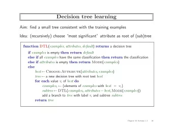
Constructing a decision tree } Function FindTree(S,A) S: samples, A: attributes } If empty(A) or all labels of the samples in S are the same status = leaf } class = most common class in the labels of S } } else status = internal } a ← bestAttribute(S,A) } LeftNode = FindTree(S(a=1),A \ {a}) } RightNode = FindTree(S(a=0),A \ {a}) } } end } end Recursive calls to create left and right subtrees S(a=1) is the set of samples in S for which a=1 9 Top down, Greedy, No backtrack

Constructing a decision tree } Function FindTree(S,A) S: samples, A: attributes } If empty(A) or all labels of the samples in S are the same status = leaf } class = most common class in the labels of S } } else status = internal } a ← bestAttribute(S,A) } LeftNode = FindTree(S(a=1),A \ {a}) } RightNode = FindTree(S(a=0),A \ {a}) Tree is constructed by splitting samples into subsets based on an } attribute value test in a recursive manner } end } end • The recursion is completed when all members of the subset at Recursive calls to create left and right subtrees a node have the same label S(a=1) is the set of samples in S for which a=1 • or when splitting no longer adds value to the predictions 10 Top down, Greedy, No backtrack

ID3 • ID3 (Examples,Target_Attribute,Attributes) • Create a root node for the tree • If all examples are positive, return the single-node tree Root, with label = + • If all examples are negative, return the single-node tree Root, with label = - • If number of predicting attributes is empty then return Root, with label = most common value of the target attribute in the examples • • else • A =The Attribute that best classifies examples. • T esting attribute for Root = A. • for each possible value, 𝑤 $ , of A • Add a new tree branch below Root, corresponding to the test A = 𝑤 $ . • Let Examples( 𝑤 $ ) be the subset of examples that have the value for A • if Examples( 𝑤 $ ) is empty then below this new branch add a leaf node with label = most common target value in the examples • • else below this new branch add subtree ID3 (Examples( 𝒘 𝒋 ),Target_Attribute,Attributes – {A}) • return Root 11

Which attribute is the best? 12

Which attribute is the best? } A variety of heuristics for picking a good test } Information gain: originated with ID3 (Quinlan,1979). } Gini impurity } … } These metrics are applied to each candidate subset, and the resulting values are combined (e.g., averaged) to provide a measure of the quality of the split. 13

� Entropy 𝐼 𝑌 = − + 𝑄 𝑦 $ log 𝑄(𝑦 $ ) 4 5 ∈7 } Entropy measures the uncertainty in a specific distribution } Information theory: } 𝐼 𝑌 : expected number of bits needed to encode a randomly drawn value of 𝑌 (under most efficient code) } Most efficient code assigns −log 𝑄(𝑌 = 𝑗) bits to encode 𝑌 = 𝑗 } ⇒ expected number of bits to code one random 𝑌 is 𝐼(𝑌) 14

Entropy for a Boolean variable 𝐼(𝑌) Entropy as a measure of impurity 𝑄(𝑌 = 1) 1 1 𝐼 𝑌 = −0.5 log < 2 − 0.5 log < 2 = 1 𝐼 𝑌 = −1 log < 1 − 0 log < 0 = 0 15

� Information Gain (IG) 𝑇 I 𝐻𝑏𝑗𝑜 𝑇, 𝐵 ≡ 𝐼 H 𝑍 − + 𝑇 𝐼 H J 𝑍 I∈KLMNOP(Q) } 𝐵 : variable used to split samples } 𝑍 : target variable } 𝑇 : samples 16

Information Gain: Example 17

� � Mutual Information } The expected reduction in entropy of 𝑍 caused by knowing 𝑌 : 𝐽 𝑌, 𝑍 = 𝐼 𝑍 − 𝐼 𝑍 𝑌 = − + + 𝑄 𝑌 = 𝑗, 𝑍 = 𝑘 log 𝑄 𝑌 = 𝑗 𝑄(𝑍 = 𝑘) 𝑄 𝑌 = 𝑗, 𝑍 = 𝑘 $ T } Mutual information in decision tree: } 𝐼 𝑍 : Entropy of 𝑍 (i.e., labels) before splitting samples } 𝐼 𝑍 𝑌 : Entropy of 𝑍 after splitting samples based on attribute 𝑌 } It shows expectation of label entropy obtained in different splits (where splits are formed based on the value of attribute 𝑌 ) 18

� � � � Conditional entropy 𝐼 𝑍 𝑌 = − + + 𝑄 𝑌 = 𝑗, 𝑍 = 𝑘 log 𝑄 𝑍 = 𝑘|𝑌 = 𝑗 $ T 𝐼 𝑍 𝑌 = + 𝑄 𝑌 = 𝑗 + −𝑄 𝑍 = 𝑘|𝑌 = 𝑗 log 𝑄 𝑍 = 𝑘|𝑌 = 𝑗 $ T probability of following i-th value for 𝑌 Entropy of 𝑍 for samples with 𝑌 = 𝑗 19

Conditional entropy: example } 𝐼 𝑍 𝐼𝑣𝑛𝑗𝑒𝑗𝑢𝑧 } = [ \] ×𝐼 𝑍 𝐼𝑣𝑛𝑗𝑒𝑗𝑢𝑧 = 𝐼𝑗𝑕ℎ + [ \] ×𝐼 𝑍 𝐼𝑣𝑛𝑗𝑒𝑗𝑢𝑧 = 𝑂𝑝𝑠𝑛𝑏𝑚 } 𝐼 𝑍 𝑋𝑗𝑜𝑒 } = g \] ×𝐼 𝑍 𝑋𝑗𝑜𝑒 = 𝑋𝑓𝑏𝑙 + j \] ×𝐼 𝑍 𝑋𝑗𝑜𝑒 = 𝑇𝑢𝑠𝑝𝑜𝑕 20

How to find the best attribute? } Information gain as our criteria for a good split } attribute that maximizes information gain is selected } When a set of 𝑇 samples have been sorted to a node, choose 𝑘 -th attribute for test in this node where: 𝑘 = argmax 𝐻𝑏𝑗𝑜 𝑇, 𝑌 $ $∈oOpLqrqrs LttP. = argmax 𝐼 H 𝑍 − 𝐼 H 𝑍|𝑌 $ } $∈oOpLqrqrs LttP. } = argmin 𝐼 H 𝑍|𝑌 $ $∈oOpLqrqrs LttP. 21

Information Gain: Example 22

ID3 algorithm: Properties } The algorithm } either reaches homogenous nodes } or runs out of attributes } Guaranteed to find a tree consistent with any conflict-free training set } ID3 hypothesis space of all DTs contains all discrete-valued functions } Conflict free training set: identical feature vectors always assigned the same class } But not necessarily find the simplest tree (containing minimum number of nodes). } a greedy algorithm with locally-optimal decisions at each node (no backtrack). 23

Decision tree learning: Function approximation problem } Problem Setting : } Set of possible instances 𝑌 } Unknown target function 𝑔: 𝑌 → 𝑍 ( 𝑍 is discrete valued) } Set of function hypotheses 𝐼 = { ℎ | ℎ ∶ 𝑌 → 𝑍 } } ℎ is a DT where tree sorts each 𝒚 to a leaf which assigns a label 𝑧 } Input : } Training examples {(𝒚 $ , 𝑧 $ )} of unknown target function 𝑔 } Output : } Hypothesis ℎ ∈ 𝐼 that best approximates target function 𝑔 24

Decision tree hypothesis space } Suppose attributes are Boolean } Disjunction of conjunctions } Which trees to show the following functions? } 𝑧 = 𝑦 \ 𝑏𝑜𝑒 𝑦 ~ } 𝑧 = 𝑦 \ 𝑝𝑠 𝑦 ] } 𝑧 = (𝑦 \ 𝑏𝑜𝑒 𝑦 ~ ) 𝑝𝑠(𝑦 < 𝑏𝑜𝑒 ¬𝑦 ] ) ? 25

Decision tree as a rule base } Decision tree = a set of rules } Disjunctions of conjunctions on the attribute values } Each path from root to a leaf = conjunction of attribute tests } All of the leafs with 𝑧 = 𝑗 are considered to find the rule for 𝑧 = 𝑗 26

How partition instance space? } Decision tree } Partition the instance space into axis-parallel regions, labeled with class value [Duda & Hurt ’s Book] 27

ID3 as a search in the space of trees } ID3 : heuristic search through space of DTs } Performs a simple to complex hill-climbing search (begins with empty tree) } prefers simpler hypotheses due to using IG as a measure of selecting attribute test } IG gives a bias for trees with minimal size. } ID3 implements a search (preference) bias instead of a restriction bias. 28