Decision Tree and Automata Learning Stefan Edelkamp 1 Overview - - PowerPoint PPT Presentation
Decision Tree and Automata Learning Stefan Edelkamp 1 Overview - Decision tree representation - Top Down Induction, Attribute Selection - Entropy, Information gain - ID3 learning algorithm - Overfitting - Continous, multi-valued, costly and
Decision Tree and Automata Learning Stefan Edelkamp
1 Overview - Decision tree representation - Top Down Induction, Attribute Selection - Entropy, Information gain - ID3 learning algorithm - Overfitting - Continous, multi-valued, costly and unkown costs - Grammar and DFA Learning - Angluin’s ID algorithm Overview 1
2 Decision Tree Learning PlayTennis: Outlook Rain Sunny Overcast Humidity Wind Yes High Normal Strong Weak No Yes No Yes Decision Tree Learning 2
Training Examples: Day Outlook Temp. Humidity Wind Play? D1 Sunny Hot High Weak No D2 Sunny Hot High Strong No D3 Overcast Hot High Weak Yes D4 Rain Mild High Weak Yes D5 Rain Cool Normal Weak Yes D6 Rain Cool Normal Strong No D7 Overcast Cool Normal Strong Yes D8 Sunny Mild High Weak No D9 Sunny Cool Normal Weak Yes D10 Rain Mild Normal Weak Yes D11 Sunny Mild Normal Strong Yes D12 Overcast Mild High Strong Yes D13 Overcast Hot Normal Weak Yes D14 Rain Mild High Strong No Decision Tree Learning 3
Decision Trees DT Representation: internal node tests attribute, branch corresponds to attribute value, leaf node assigns classification When to consider DT: - Instances describable by attribute–value pairs - Target function discrete valued - Disjunctive hypothesis may be required - Possibly noisy training data Examples: Equipment or medical diagnosis, Credit risk analysis, modeling calendar scheduling preferences Decision Tree Learning 4
Top-Down Induction Main Loop: A “best” decision attribute for next node , assign A as decision attribute for node - for each value of A , create new descendant of node - sort training examples to leaf nodes if training examples perfectly classified ⇒ stop else iterate over new leaf nodes Best Attribute: A1=? A2=? [29+,35-] [29+,35-] t f t f [21+,5-] [8+,30-] [18+,33-] [11+,2-] Decision Tree Learning 5
Entropy 1.0 Entropy(S) 0.5 0.0 0.5 1.0 p + - S is a sample of training examples p ⊕ : proportion of positive examples in S , p ⊖ : proportion of negative examples in S Entropy measures the impurity of S Entropy ( S ) ≡ − p ⊕ log 2 p ⊕ − p ⊖ log 2 p ⊖ = expected # bits needed to encode class ( ⊕ or ⊖ ) of randomly drawn member of S (under the optimal, shortest-length code) Decision Tree Learning 6
Selecting the Next Attribute Information Gain: expected reduction in entropy due to sorting on A | S v | � Gain ( S, A ) ≡ Entropy ( S ) − | S | Entropy ( S v ) v ∈ D A Which attribute is the best classifier? S: [9+,5-] S: [9+,5-] E =0.940 E =0.940 Humidity Wind High Normal Weak Strong [3+,4-] [6+,1-] [6+,2-] [3+,3-] E =0.985 E =0.592 E =0.811 E =1.00 Gain (S, Humidity ) Gain (S, ) Wind = .940 - (7/14).985 - (7/14).592 = .940 - (8/14).811 - (6/14)1.0 = .151 = .048 Decision Tree Learning 7
ID3: Hypothesis Space Search + – + ... A2 A1 + – + – + – + + � ... A2 A2 + – + – + – + – A4 A3 – + ... ... Target Function: surely in there . . . , no backtracking ⇒ Local minima . . . Statistical Choices: robust to noisy data, inductive bias: “prefer shortest tree” Decision Tree Learning 8
Occam’s Razor Bias: preference for some hypotheses, rather than a restriction of hypothesis space . . . prefershortest hypothesis that fits the data Arguments in favor to short hypotheses: - a short hyp that fits data unlikely to be coincidence, a long hyp that fits data likely be coincidence Arguments opposed short hypotheses: - There are many ways to define small sets of hyps, e.g., all trees with a prime number of nodes that use attributes beginning with “Z” - What’s so special about small sets based on size of hypothesis? Decision Tree Learning 9
Overfitting in Decision Trees Consider adding noisy Sunny, Hot, Normal, Strong, PlayTennis = No Consider error of hypothesis h over - training data: error train ( h ) - entire distribution D of data: error D ( h ) Hypothesis h ∈ H overfits training data if there is an alternative hypothesis h ′ ∈ H such that error train ( h ) < error train ( h ′ ) and error D ( h ) > error D ( h ′ ) Decision Tree Learning 10
0.9 0.85 0.8 0.75 Accuracy 0.7 0.65 0.6 On training data On test data 0.55 0.5 0 10 20 30 40 50 60 70 80 90 100 Size of tree (number of nodes)
Avoiding Overfitting Option 1: stop growing when split not statistically significant Option 2: grow full tree, then post-prune Select best tree: - measure performance over training data - measure performance over separate validation data set - min. | tree | + | misclassifications ( tree ) | Decision Tree Learning 11
Rule Post-Pruning - Convert tree to equivalent set of rules - Prune each rule independently of others - Sort final rules into desired sequence for use Perhaps most frequently used method Decision Tree Learning 12
Converting A Tree to Rules Outlook Sunny Overcast Rain Humidity Wind Yes High Normal Strong Weak No Yes No Yes ( Outlook = Sunny ) ∧ ( Humidity = High ) IF THEN PlayTennis = No IF ( Outlook = Sunny ) ∧ ( Humidity = Normal ) THEN PlayTennis = Y es . . . Decision Tree Learning 13
Continuous Valued Attributes Create a discrete attribute to test continuous ( Temperature > 72 . 3) = t, f Temperature : 40 48 60 72 80 90 PlayTennis : No No Yes Yes Yes No Attributes with Many Values: Gain will select it e.g. Date = Jun 3 1996 One approach: use Gain ( S, A ) GainRatio ( S, A ) ≡ SplitInformation ( S, A ) c | S i | | S i | � SplitInformation ( S, A ) ≡ − | S | log 2 | S | i =1 where S i is subset of S for which A has value v i Decision Tree Learning 14
Attributes with Costs e.g medical diagnosis: BloodTest has costs Consistent tree with low expected cost: replace gain by - Gain 2 ( S, A ) /Cost ( A ) . - 2 Gain ( S,A ) − 1 / ( Cost ( A ) + 1) w m , where w ∈ [0 , 1] determines importance of cost Decision Tree Learning 15
Unknown Attribute Values Use training example anyway, sort through tree - node n tests A ⇒ assign most common value of A among other examples sorted to node n - assign most common value of A among other examples with same target value - assign probability p i to each possible value v i of A - assign fraction p i of example to each descendant Classify new examples in same fashion Decision Tree Learning 16
3 Automata Learning Grammar Inference: process of learning an unknown grammar given a finite set of labeled examples Regular Grammar: recognized by DFA Given: finite set of positive examples, finite, possibly empty set of negative examples Task: learn minimum state DFA equivalent to target . . . is NP-hard Simplifications: - criteria on samples (e.g. structural completeness) - knowledgeable teacher (oracle) who responds to queries generated by learner Automata Learning 17
Applications - Inference of control structures in learning by examples - Inference of normal models of systems in test - Inference of consistent environments in partial models Automata Learning 18
Trace Tree Automata Learning 19
DFA Automata Learning 20
Chart Parsing Automata Learning 21
Chart Parsing Automata Learning 22
Chart Parsing Automata Learning 23
Chart Parsing Automata Learning 24
Chart Parsing Automata Learning 25
Some Notation Σ : set of symbols, Σ ∗ : set of strings , λ : empty string M = ( Q, δ, Σ , q 0 , F ) : DFA, L ( M ) : language accepted by M q in M alive: to be reached by some string α and left with some string β such that αβ ∈ L ( M ) ⇒ in minimal DFA only one non-alive state d 0 set of strings P live-complete w.r.t. M : ∀ live states q in M : ∃ α ∈ P with δ ( q 0 , α ) = q ⇒ P ′ = P ∪ { d 0 } represents all states in M f : P ′ × Σ → Σ ∗ ∪ { d 0 } by f ( d 0 , b ) = d 0 and f ( α, b ) = αb Transition set T ′ : P ′ ∪ { f ( α, b ) | ( α, b ) ∈ P × Σ } ; T = T ′ − { d 0 } Automata Learning 26
Angluin’s ID-Algorithm Aim: construct a partition of T ′ that places all the equivalent elements in one state Equivalence relation: Nerode ⇒ DFA minimal Start: one accepting and one non-accepting state Partitioning: - ∀ i string v i is drawn, s.t. ∀ q, q ′ ∃ j ≤ i with δ ( q, v j ) ∈ F and δ ( q ′ , v j ) / ∈ F , or vice versa ⇒ i -th partition E i : E i ( d 0 ) = ∅ and E i ( α ) = { v j | j ≤ i, αv j ∈ L ( M ) } - ∀ α, β ∈ T with δ ( q 0 , α ) = δ ( q 0 , β ) we have E j ( α ) = E j ( β ) , j ≤ i Automata Learning 27
Construct ( i + 1) -th Partition Separation: - ∀ i search α, β and b s.t. E i ( α ) = E i ( β ) but E i ( f ( α, b )) � = E i ( f ( β, b )) γ : element in E i ( f ( α, b )) and not in E i ( f ( β, b )) or vice versa ∀ α ∈ T : query the string αv i +1 , v i +1 = bγ αv i +1 ∈ L ( M ) ⇒ E i +1 ← E i ∪ { v i +1 } ; otherwise, E i +1 ← E i . . . iterate until no separating pair α , β exists Automata Learning 28
Recommend
More recommend
Explore More Topics
Stay informed with curated content and fresh updates.
