Decision Trees MAT 6480W / STT 6705V Guy Wolf - PowerPoint PPT Presentation
Geometric Data Analysis Decision Trees MAT 6480W / STT 6705V Guy Wolf guy.wolf@umontreal.ca Universit e de Montr eal Fall 2019 MAT 6480W (Guy Wolf) Decision Trees UdeM - Fall 2019 1 / 15 Outline Decision Trees 1 Hunts
Geometric Data Analysis Decision Trees MAT 6480W / STT 6705V Guy Wolf guy.wolf@umontreal.ca Universit´ e de Montr´ eal Fall 2019 MAT 6480W (Guy Wolf) Decision Trees UdeM - Fall 2019 1 / 15
Outline Decision Trees 1 Hunt’s algorithm Node splitting Impurity measures Decision boundaries Tree pruning Random forests 2 Ensemble of decision trees Randomization approaches Random projections 3 Johnson-Lindenstrauss lemma Sparse random projections MAT 6480W (Guy Wolf) Decision Trees UdeM - Fall 2019 2 / 15
Decision trees A decision tree is a simple, yet effective model, for classification. The tree induction step essentially builds a set of IF-THEN rules , which can be visualized as a tree, for testing class membership of data points. The deduction step tests these conditions and follows the branches of the tree to establish class membership Intuitively, this can be thought of as building an “interview” for estimating the classification of each data point. MAT 6480W (Guy Wolf) Decision Trees UdeM - Fall 2019 3 / 15
Decision trees MAT 6480W (Guy Wolf) Decision Trees UdeM - Fall 2019 3 / 15
Decision trees MAT 6480W (Guy Wolf) Decision Trees UdeM - Fall 2019 3 / 15
Decision trees Tree building algorithms Over the years many decision tree (induction) algorithms have been proposed. Examples (Decision tree induction algorithms) CART (Classification And Regression Trees) ID3 (Iterative Dichotomiser 3) & C4.5 SLIQ & SPRINT Rainforest & BOAT Most of them follow a basic top-down paradigm known as Hunt’s Al- gorithm, although some use alternative approaches (e.g., bottom-up constructions) and particular implementation steps to improve perfor- mances. MAT 6480W (Guy Wolf) Decision Trees UdeM - Fall 2019 4 / 15
Decision trees Basic approach (Hunt’s algorithm) A tree is constructed top-down using a recursive greedy approach: Start with all the training samples at the root 1 Choose the best attribute & split into several data subsets 2 Create a branch & child node for each subset 3 Run the algorithm recursively for each child node and associated 4 subset Stop the recursion when one of the following conditions are met: 5 All the data points in the node have the same class label There are no attributes left to split by The node is empty If a leaf node contains more than one class label, use majority/plurality voting to set its class. MAT 6480W (Guy Wolf) Decision Trees UdeM - Fall 2019 5 / 15
Decision trees Basic approach (Hunt’s algorithm) MAT 6480W (Guy Wolf) Decision Trees UdeM - Fall 2019 5 / 15
Decision trees Node splitting Each internal node in the tree considers: a subset of the data, based on the path leading to it an attribute to test and generate smaller subsets to pass to child nodes Splitting a node to child nodes depends on the type of the tested attribute and the configuration of the algorithm. For example, some algorithms force binary splits (e.g.,CART), while others allow multiway splits (e.g, C4.5). MAT 6480W (Guy Wolf) Decision Trees UdeM - Fall 2019 6 / 15
Decision trees Node splitting Splitting nominal attributes: Binary splits: use a set of possible values on one branch and its complement on the other: or Multiway splits: use a separate branch for each possible value: MAT 6480W (Guy Wolf) Decision Trees UdeM - Fall 2019 6 / 15
Decision trees Node splitting Splitting ordinal attributes: Binary splits: find a threshold and partition into values above and below it: or Multiway splits: use a separate branch for each possible value: MAT 6480W (Guy Wolf) Decision Trees UdeM - Fall 2019 6 / 15
Decision trees Node splitting Splitting numerical attributes: Binary splits: find a threshold and partition into values above and below it: Multiway splits: Discretize the values (statically as preprocessing or dynamically) to form ordinal values: MAT 6480W (Guy Wolf) Decision Trees UdeM - Fall 2019 6 / 15
Decision trees Node splitting How do we choose the best attribute (and split) to use at each node? We want to increase the homogeneity and reduce heterogeneity in the resulting subnodes. In other words - we want subsets that are as pure as possible w.r.t. class labels. MAT 6480W (Guy Wolf) Decision Trees UdeM - Fall 2019 6 / 15
Decision trees Impurity measures MAT 6480W (Guy Wolf) Decision Trees UdeM - Fall 2019 7 / 15
Decision trees Impurity measures Impurity can be quantified in several ways, which vary from one algorithm to another: Impurity measures Misclassification error Entropy (e.g., ID3 and C4.5) Gini index (e.g., CART, SLIQ, and SPRINT) In general, these measures are equivalent in most cases, but there are specific cases when one can be advantageous over others. MAT 6480W (Guy Wolf) Decision Trees UdeM - Fall 2019 7 / 15
Decision trees Impurity measures Impurity can be quantified in several ways, which vary from one algorithm to another: Impurity measures Misclassification error Entropy (e.g., ID3 and C4.5) Gini index (e.g., CART, SLIQ, and SPRINT) The impurity gain of a split t �→ t 1 , . . . , t k is the difference #pts( t i ) � ∆ Impurity = Impurity( t ) − #pts( t ) Impurity( t i ) i =1 between impurity at t and a weighted average of child impurities. MAT 6480W (Guy Wolf) Decision Trees UdeM - Fall 2019 7 / 15
Decision trees Impurity measures Misclassification error The error rate incurred by classifying the entire node by plurality vote: Error( t ) = 1 − max c { p ( c | t ) } where p ( c | t ) is the frequency of class c in node t . Minimum error is zero - achieved when all data points in the node have the same class 1 Maximum error is 1 − #classes - achieved when data points in the node are equally distributed between the classes MAT 6480W (Guy Wolf) Decision Trees UdeM - Fall 2019 7 / 15
Decision trees Impurity measures Examples (Misclassification error) MAT 6480W (Guy Wolf) Decision Trees UdeM - Fall 2019 7 / 15
Decision trees Impurity measures Misclassification error does not always detect improvements: Example MAT 6480W (Guy Wolf) Decision Trees UdeM - Fall 2019 7 / 15
Decision trees Impurity measures Entropy A standard information-theoretic concept that measures the impurity of a node based on the amount “bits” required to represent the class labels in it: � Entropy( t ) = − p ( c | t ) log 2 p ( c | t ) c where p ( c | t ) is the frequency of class c in node t . Minimum entropy is zero - achieved when all data points in the node have the same class Maximum entropy is log(#classes) - achieved when data points in the node are equally distributed between the classes MAT 6480W (Guy Wolf) Decision Trees UdeM - Fall 2019 7 / 15
Decision trees Impurity measures Examples (Entropy) MAT 6480W (Guy Wolf) Decision Trees UdeM - Fall 2019 7 / 15
Decision trees Impurity measures Information Gain For a node t split into child nodes t 1 , . . . , t k , the information gain of this split is defined as: #pts( t i ) � Info Gain( t , t 1 , . . . , t k ) = Entropy( t ) − #pts( t ) Entropy( t i ) i =1 where #pts( · ) is the number of data points in a node. Measures the reduction in Entropy achieved by the split - an optimal split would maximize this gain. Disadvantage: tends to prefer large number of small pure child nodes (e.g., may cause overfitting) MAT 6480W (Guy Wolf) Decision Trees UdeM - Fall 2019 7 / 15
Decision trees Impurity measures Gain Ratio For a node t split into child nodes t 1 , . . . , t k , the gain ratio normalizes the information gain by k #pts( t i ) #pts( t i ) � Split Info( t , t 1 , . . . , t k ) = − #pts( t ) log 2 #pts( t ) i =1 to get Gain Ratio = Info Gain Split Info . Penalizes high-entropy partitions (i.e., with large number of small child nodes) Used in C4.5 to overcome the disadvantage of raw information gain. MAT 6480W (Guy Wolf) Decision Trees UdeM - Fall 2019 7 / 15
Decision trees Impurity measures Gini index A “social inequality” (or, more formally, statistical dispersion) index developed by the statistician/sociologist Corrado Gini: [ p ( c | t )] 2 � Gini( t ) = 1 − c where p ( c | t ) is the frequency of class c in node t . Minimum Gini value is zero - achieved when all data points in the node have the same class 1 Maximum Gini index is 1 − #classes - achieved when data points in the node are equally distributed between the classes MAT 6480W (Guy Wolf) Decision Trees UdeM - Fall 2019 7 / 15
Decision trees Impurity measures Examples (Gini index) MAT 6480W (Guy Wolf) Decision Trees UdeM - Fall 2019 7 / 15
Decision trees Impurity measures Gini for a split is computed similarly to misclassification error, but does better: Example MAT 6480W (Guy Wolf) Decision Trees UdeM - Fall 2019 7 / 15
Decision trees Impurity measures Comparison of the three impurity measures for two classes, where p is the portion of points in the first class (and 1 − p in the other class): MAT 6480W (Guy Wolf) Decision Trees UdeM - Fall 2019 7 / 15
Recommend
More recommend
Explore More Topics
Stay informed with curated content and fresh updates.
