Decision Sequence Matrix Multiplication Chains Determine the best - PDF document

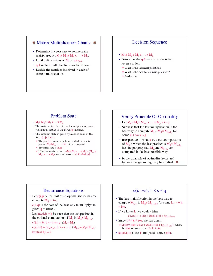
Decision Sequence Matrix Multiplication Chains • Determine the best way to compute the • M 1 x M 2 x M 3 x … x M q matrix product M 1 x M 2 x M 3 x … x M q . • Determine the q-1 matrix products in • Let the dimensions of M i be r i x r i+1 . reverse order. • q-1 matrix multiplications are to be done. � What is the last multiplication? • Decide the matrices involved in each of � What is the next to last multiplication? these multiplications. � And so on. Problem State Verify Principle Of Optimality • M 1 x M 2 x M 3 x … x M q • Let M ij = M i x M i+1 x … x M j , i <= j. • The matrices involved in each multiplication are a • Suppose that the last multiplication in the contiguous subset of the given q matrices. best way to compute M ij is M ik x M k+1,j for • The problem state is given by a set of pairs of the some k, i <= k < j. form (i, j), i <= j. • Irrespective of what k is, a best computation � The pair (i,j) denotes a problem in which the matrix of M ij in which the last product is M ik x M k+1,j product M i x M i+1 x … x M j is to be computed. has the property that M ik and M k+1,j are � The initial state is (1,q). � If the last matrix product is (M 1 x M 2 x … x M k ) x (M k+1 x computed in the best possible way. M k+2 x … x M q ), the state becomes {(1,k), (k+1,q)}. • So the principle of optimality holds and dynamic programming may be applied. Recurrence Equations c(i, i+s), 1 < s < q • Let c(i,j) be the cost of an optimal (best) way to • The last multiplication in the best way to compute M ij , i <= j. compute M i,i+s is M ik x M k+1,i+s for some k, i <= k • c(1,q) is the cost of the best way to multiply the < i+s. given q matrices. • If we knew k, we could claim: • Let kay(i,j) = k be such that the last product in c(i,i+s) = c(i,k) + c(k+1,i+s) + r i r k+1 r i+s+1 the optimal computation of M ij is M ik x M k+1,j . • Since i <= k < i+s, we can claim • c(i,i) = 0, 1 <= i <= q. (M ii = M i ) c(i,i+s) = min{c(i,k) + c(k+1,i+s) + r i r k+1 r i+s+1 }, where • c(i,i+1) = r i r i+1 r i+2 , 1 <= i < q. (M ii+1 = M i x M i+1 ) the min is taken over i <= k < i+s. • kay(i,i+1) = i. • kay(i,i+s) is the k that yields above min.

Recursive Implementation Recurrence Equations • c(i,i+s) = • See text for recursive codes. min i <= k < i+s {c(i,k) + c(k+1,i+s) + r i r k+1 r i+s+1 } • Code that does not avoid recomputation of already computed c(i,j)s runs in Omega(2 q ) • c(*,*) terms on right side involve fewer matrices time. than does the c(*,*) term on the left side. • Code that does not recompute already computed • So compute in the order s = 2, 3, …, q-1. c(i,j)s runs in O(q 3 ) time. • Implement nonrecursively for best worst-case efficiency. Example s = 0 • q = 4, (10 x 1) * (1 x 10) * (10 x 1) * (1 x 10) c(i,i) and kay(i,i) , 1 <= i <= 4 are to be computed. • r = [r 1 ,r 2 ,r 3 ,r 4 ,r 5 ] = [10, 1, 10, 1, 10] 1 2 3 4 1 2 0 0 3 0 0 4 0 0 0 0 kay(i,j), i <= j c(i,j), i <= j kay(i,j), i <= j c(i,j), i <= j s = 1 s = 1 c(i,i+1) and kay(i,i+1) , 1 <= i <= 3 are to be • c(i,i+1) = r i r i+1 r i+2 , 1 <= i < q. (M ii+1 = M i x M i+1 ) computed. • kay(i,i+1) = i. • r = [r 1 ,r 2 ,r 3 ,r 4 ,r 5 ] = [10, 1, 10, 1, 10] 0 0 1 0 0 100 0 0 2 0 0 10 0 0 3 0 0 100 0 0 0 0 kay(i,j), i <= j kay(i,j), i <= j c(i,j), i <= j c(i,j), i <= j

s = 2 s = 2 • c(i,i+2) = min{c(i,i) + c(i+1,i+2) + r i r i+1 r i+3 , • c(1,3) = min{c(1,1) + c(2,3) + r 1 r 2 r 4 , c(i,i+1) + c(i+2,i+2) + r i r i+2 r i+3 } c(1,2) + c(3,3) + r 1 r 3 r 4 } • r = [r 1 ,r 2 ,r 3 ,r 4 ,r 5 ] = [10, 1, 10, 1, 10] • r = [r 1 ,r 2 ,r 3 ,r 4 ,r 5 ] = [10, 1, 10, 1, 10] • c(1,3) = min{0 + 10 + 10, 100 + 0 + 100} 0 1 0 1 1 0 100 0 100 20 0 2 0 2 0 10 0 10 0 3 0 3 0 100 0 100 0 0 0 0 kay(i,j), i <= j kay(i,j), i <= j c(i,j), i <= j c(i,j), i <= j s = 2 s = 3 • c(2,4) = min{c(2,2) + c(3,4) + r 2 r 3 r 5 , • c(1,4) = min{c(1,1) + c(2,4) + r 1 r 2 r 5 , c(2,3) + c(4,4) + r 2 r 4 r 5 } c(1,2) + c(3,4) + r 1 r 3 r 5 , c(1,3) + c(4,4) + r 1 r 4 r 5 } • r = [r 1 ,r 2 ,r 3 ,r 4 ,r 5 ] = [10, 1, 10, 1, 10] • r = [r 1 ,r 2 ,r 3 ,r 4 ,r 5 ] = [10, 1, 10, 1, 10] • c(2,4) = min{0 + 100 + 100, 10 + 0 + 10} • c(1,4) = min{0+20+100, 100+100+1000, 20+0+100} 0 1 1 0 1 1 1 0 100 20 0 100 20 120 0 2 3 0 2 3 0 10 20 0 10 20 0 3 0 3 0 100 0 100 0 0 0 0 kay(i,j), i <= j kay(i,j), i <= j c(i,j), i <= j c(i,j), i <= j Determine The Best Way To Compute M 14 Determine The Best Way To Compute M 24 • kay(1,4) = 1. • kay(2,4) = 3 . • So the last multiplication is M 14 = M 11 x M 24 . • So the last multiplication is M 24 = M 23 x M 44 . • M 11 involves a single matrix and no multiply. • M 23 = M 22 x M 33 . • Find best way to compute M 24 . • M 44 involves a single matrix and no multiply. 0 1 1 1 0 1 1 1 0 100 20 120 0 100 20 120 0 2 3 0 2 3 0 10 20 0 10 20 0 3 0 3 0 100 0 100 0 0 0 0 kay(i,j), i <= j kay(i,j), i <= j c(i,j), i <= j c(i,j), i <= j

Time Complexity The Best Way To Compute M 14 1 2 3 4 1 0 100 20 120 c(i,j), i <= j 2 0 10 20 0 100 • The multiplications (in reverse order) are: 3 0 4 � M 14 = M 11 x M 24 • O(q 2 ) c(i,j) values are to be computed, where q is the � M 24 = M 23 x M 44 number of matrices. � M 23 = M 22 x M 33 • c(i,i+s) = min i <= k < i+s {c(i,k) + c(k+1,i+s) + r i r k+1 r i+s+1 }. • Each c(i,j) is the min of O(q) terms. • Each of these terms is computed in O(1) time. • So all c(i,j) are computed in O(q 3 ) time. Time Complexity 1 2 3 4 1 0 1 1 1 kay(i,j), i <= j 2 0 2 3 0 3 3 0 4 • The traceback takes O(1) time to determine each matrix product that is to be done. • q-1 products are to be done. • Traceback time is O(q).