Parallel Scientific Computing Matrix-vector multiplication. - PDF document

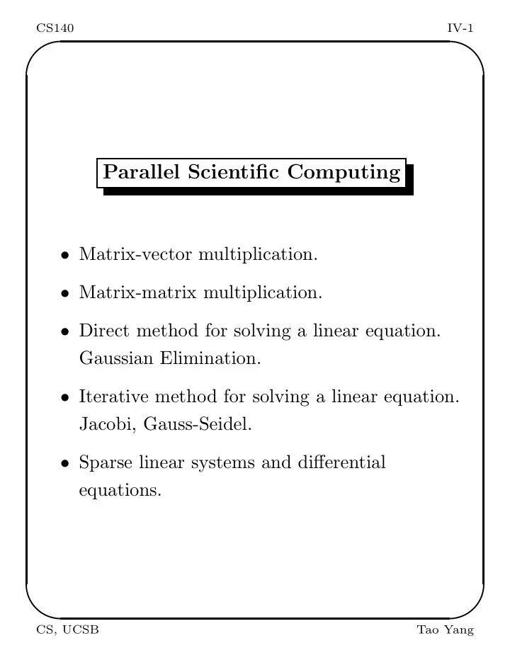
✬ ✩ CS140 IV-1 Parallel Scientific Computing • Matrix-vector multiplication. • Matrix-matrix multiplication. • Direct method for solving a linear equation. Gaussian Elimination. • Iterative method for solving a linear equation. Jacobi, Gauss-Seidel. • Sparse linear systems and differential equations. ✫ ✪ CS, UCSB Tao Yang

✬ ✩ CS140 IV-2 Iterative Methods for Solving Ax = b Ex: (1) 6 x 1 − 2 x 2 + x 3 = 11 (2) − 2 x 1 + 7 x 2 + 2 x 3 = 5 (3) x 1 + 2 x 2 − 5 x 3 = -1 = ⇒ 11 6 − 1 x 1 = 6 ( − 2 x 2 + x 3 ) 7 − 1 5 x 2 = 7 ( − 2 x 1 + 2 x 3 ) 1 1 x 3 = 5 − − 5 ( x 1 + 2 x 2 ) = ⇒ x ( k +1) 6 (11 − ( − 2 x ( k ) + x ( k ) 1 = 3 )) 1 2 x ( k +1) 7 (5 − ( − 2 x ( k ) + 2 x ( k ) 1 = 3 )) 2 1 x ( k +1) − 5 ( − 1 − ( x ( k ) + 2 x ( k ) 1 = 2 )) 3 1 ✫ ✪ CS, UCSB Tao Yang

✬ ✩ CS140 IV-3 Initial Approximation: x 1 = 0 , x 2 = 0 , x 3 = 0 Iter 0 1 2 3 4 · · · 8 x 1 0 1.833 2.038 2.085 2.004 · · · 2.000 x 2 0 0.714 1.181 1.053 1.001 · · · 1.000 x 3 0 0.2 0.852 1.080 1.038 · · · 1.000 x ( k +1) − � x ( k ) � < 10 − 4 Stop when � � x ( k +1) − � x ( k ) � . Need to define norm � � ✫ ✪ CS, UCSB Tao Yang

✬ ✩ CS140 IV-4 Iterative methods in a matrix format k +1 k         2 − 1 11 x 1 0 x 1 6 6 6         2 − 2 5 = + x 2 0 x 2         7 7 7                 1 2 1 x 3 0 x 3 5 5 5 General iterative method: x (0) Assign an initial value to � k=0 Do x ( k +1) = H ∗ � x ( k ) + d � x ( k +1) − � x ( k ) � < ε until � � ✫ ✪ CS, UCSB Tao Yang

✬ ✩ CS140 IV-5 Norm of a Vector Given x = ( x 1 , x 2 , · · · x n ): n � � x � 1 = | x i | i =1 �� | x i | 2 � x � 2 = � x � ∞ = max | x i | Example: x = ( − 1 , 1 , 2) � x � 1 = 4 √ 1 + 1 + 2 2 = � � x � 2 = 6 � x � ∞ = 2 Applications: � Error �≤ ε ✫ ✪ CS, UCSB Tao Yang

✬ ✩ CS140 IV-6 Jacobi Method for Ax = b = 1 x k +1 � a ij x k ( b i − j ) i = 1 , · · · n i a ii j � = i Example: (1) 6 x 1 − 2 x 2 + x 3 = 11 (2) − 2 x 1 + 7 x 2 + 2 x 3 = 5 (3) x 1 + 2 x 2 − 5 x 3 = -1 = ⇒ 11 6 − 1 x 1 = 6 ( − 2 x 2 + x 3 ) 5 7 − 1 x 2 = 7 ( − 2 x 1 + 2 x 3 ) 1 1 x 3 = 5 − − 5 ( x 1 + 2 x 2 ) ✫ ✪ CS, UCSB Tao Yang

✬ ✩ CS140 IV-7 Jacobi method in a matrix-vector form k +1 k         2 − 1 11 x 1 0 x 1 6 6 6         2 − 2 5 = + x 2 0 x 2         7 7 7                 1 2 1 x 3 0 x 3 5 5 5 ✫ ✪ CS, UCSB Tao Yang

✬ ✩ CS140 IV-8 Parallel Jacobi Method x k +1 = D − 1 Bx k + D − 1 b or in general x k +1 = Hx k + d. Parallel solution: • Distribute rows of H to processors. • Perform computation based on owner-computes rule. • Perform all-gather collective communication after each iteration. ✫ ✪ CS, UCSB Tao Yang

✬ ✩ CS140 IV-9 Task graph/schedule for y = H ∗ x + d Partitioned code: for i = 1 to n do S i : y i = 0; for j = 1 to n do y i = y i + H i,j ∗ x j + d j ; endfor endfor Task graph: S3 S2 S1 Sn Schedule: 0 p−1 1 Sr+1 S1 S2 Sr+2 Sn S2r Sr ✫ ✪ CS, UCSB Tao Yang

✬ ✩ CS140 IV-10 Data Mapping for H ∗ x + d Block Mapping function of tasks S i : proc map ( i ) = ⌊ i − 1 r ⌋ where r = ⌈ n p ⌉ . Data partitioning: Matrix H is divided into n rows H 1 , H 2 , · · · H n . Data mapping : Row H i is mapped to processor proc map ( i ). Vectors y and d are distributed in the same way. Vector x is replicated to all processors. Local indexing function is: local ( i ) = ( i − 1) mod r . ✫ ✪ CS, UCSB Tao Yang

✬ ✩ CS140 IV-11 SPMD Code for y = H ∗ x + d me=mynode(); for i = 1 to n do if proc map ( i ) == me , then do S i : S i : y [ i ] = 0; i 1 = Local ( i ) for j = 1 to n do y [ i 1] = y [ i 1] + a [ i 1][ j ] ∗ x [ j ] + d [ i 1] endfor endfor ✫ ✪ CS, UCSB Tao Yang

✬ ✩ CS140 IV-12 Cost of Jacobi Method Space cost per processor is O ( n 2 /p ) Time cost: • T is the number of iterations. • The all-gather time cost per iteration is C . Proc 0 x0 Proc 0 x0 Proc 1 Proc 1 x1 x1 Proc 2 Proc 2 x2 x2 Proc 3 Proc 3 x3 x3 (a) Gather (b) All Gather • Main cost of S i : 2 n multiplication and addition (2 nω ). • Overhead of loop control and code mapping can be reduced, and becomes less significant. The parallel time is PT ≈ T ( n p × 2 nω + C ) = O ( T ( n 2 /p + C )) . ✫ ✪ CS, UCSB Tao Yang

✬ ✩ CS140 IV-13 Optimizing SPMD Code: Example SPMP code with block mapping: me=mynode(); For i =0 to rp-1 if ( proc map ( i ) == me ) a[Local(i)] = 3. Remove extra loop and branch overhead. me=mynode(); For i = r*me to r*me+r-1 a[Local(i)] = 3. Further simplification on distributed memory machines me=mynode(); For s = 0 to r-1 a[s] = 3. ✫ ✪ CS, UCSB Tao Yang

✬ ✩ CS140 IV-14 If the iterative matrix H is sparse If it contains a lot of zeros, the code design should take advantage of this: • Not store too many known zeros. • Code should explicitly skip those operations applied to zero elements. Example: y 0 = y n +1 = 0. y 0 − 2 y 1 + y 2 = h 2 y 1 − 2 y 2 + y 3 = h 2 . . . y n − 1 − 2 y n + y n +1 = h 2 ✫ ✪ CS, UCSB Tao Yang

✬ ✩ CS140 IV-15 This set of equations can be rewritten as:       h 2 − 2 1 y 1       h 2  1 − 2 1   y 2                . . . .       = 1 − 2 1 . .             ...       h 2 1 y n − 1                   h 2 1 − 2 y n The Jacobi method in a matrix format (right side): k       h 2 0 1 y 1       h 2  1 0 1   y 2                . . . .       0 . 5 ∗ − 0 . 5 ∗ 1 0 1 . .             ...       h 2 1 y n − 1                   h 2 1 0 y n Too time and space consuming if you multiply using the entire iterative matrix! ✫ ✪ CS, UCSB Tao Yang

✬ ✩ CS140 IV-16 Optimized solution: write the Jacobi method as: Repeat For i = 1 to n i +1 − h 2 ) y new = 0 . 5( y old i − 1 + y old i Endfor y new − � y old � < ε Until � � ✫ ✪ CS, UCSB Tao Yang

✬ ✩ CS140 IV-17 Gauss-Seidel Method Utilize new solutions as soon as they are available. (1) 6 x 1 − 2 x 2 + x 3 = 11 (2) − 2 x 1 + 7 x 2 + 2 x 3 = 5 (3) x 1 + 2 x 2 − 5 x 3 = -1 = ⇒ Jacobi method. x k +1 1 6 (11 − ( − 2 x k 2 + x k = 3 )) 1 x k +1 1 7 (5 − ( − 2 x k 1 + 2 x k = 3 )) 2 x k +1 1 − 5 ( − 1 − ( x k 1 + 2 x k = 2 )) 3 = ⇒ Gauss-Seidel method. x k +1 1 6 (11 − ( − 2 x k 2 + x k = 3 )) 1 x k +1 7 (5 − ( − 2 x k +1 1 + 2 x k = 3 )) 2 1 x k +1 − 5 ( − 1 − ( x k +1 + 2 x k +1 1 = )) 3 1 2 ✫ ✪ CS, UCSB Tao Yang

✬ ✩ CS140 IV-18 ε = 10 − 4 0 1 2 3 4 5 x 1 0 1.833 2.069 1.998 1.999 2.000 x 2 0 1.238 1.002 0.995 1.000 1.000 x 3 0 1.062 1.015 0.998 1.000 1.000 It converges faster than Jacobi’s method. ✫ ✪ CS, UCSB Tao Yang

✬ ✩ CS140 IV-19 The SOR method SOR (Successive Over Relaxation). The rate of convergence can be improved (accelerated) by the SOR method: Step 1: Use the Gauss-Seidel Method. x k +1 = Hx k + d Step 2: x k +1 = x k + w ( x k +1 − x k ) ✫ ✪ CS, UCSB Tao Yang

✬ ✩ CS140 IV-20 Convergence of iterative methods Notation: x ∗ ↔ exact solution x k ↔ solution vector at step k Definition: Sequence x 0 , x 1 , x 2 , · · · , x n converges to the solution x ∗ with respect to norm � . � if � x k − x ∗ � < ε when k is very large. i.e. k → ∞ , � x k − x ∗ �→ 0 ✫ ✪ CS, UCSB Tao Yang

✬ ✩ CS140 IV-21 A condition for convergence Let error e k = x k − x ∗ x k +1 = Hx k + d x ∗ = Hx ∗ + d x k +1 − x ∗ = H ( x k − x ∗ ) e k +1 = He ∗ � e k +1 �≤� He k �≤� H �� e k � ≤� H � 2 � e k − 1 �≤ · · · ≤� H � k +1 � e 0 � Then if � H � < 1 , = ⇒ The method converges. Need to define the matrix norm. ✫ ✪ CS, UCSB Tao Yang

✬ ✩ CS140 IV-22 Matrix Norm Given a matrix of dimension n × n , Define n � � H � ∞ = max h ij max sum row 1 ≤ i ≤ n j =1 n � � H � 1 = max h ij max sum column 1 ≤ j ≤ n i =1 Example:   5 9 H =   − 2 1 � H � ∞ = max (14 , 3) = 14 � H � 1 = max (7 , 10) = 10 ✫ ✪ CS, UCSB Tao Yang