Lecture 17/18: Dynamic Programming - Matrix Chain Parenthesization - PowerPoint PPT Presentation

Lecture 17/18: Dynamic Programming - Matrix Chain Parenthesization COMS10007 - Algorithms Dr. Christian Konrad 01.04.2019 and 02.04.2019 Dr. Christian Konrad Lecture 17/18: Matrix Chain Parenthesization 1 / 18

Matrix Multiplication Problem: Matrix-Multiplication 1 Input: Matrices A , B with A . columns = B . rows 2 Output: Matrix product A × B Example: q r     2 3 6 2 4 r q 1 0 � 0 1 2 � 0 1 2      × = p p     2 6 2 0 0 12 2 4    0 9 18 0 0 Notation: p × q matrix: p rows and q columns p × q matrix times q × r matrix gives a p × r matrix ( A × B ) i , j = row i of A times column j of B Dr. Christian Konrad Lecture 17/18: Matrix Chain Parenthesization 2 / 18

Algorithm for Matrix-Multiplication Algorithm: ( A × B ) i , j = row i of A times column j of B Require: Matrices A , B with A . columns = B . rows Let C be a new A . rows × B . columns matrix for i ← 1 . . . A . rows do for j ← 1 . . . B . columns do C ij ← 0 for k ← 1 . . . A . columns do C ij ← C ij + A ik · B kj return C Algorithm Matrix-Multiply ( A , B ) Runtime: Three nested loops: O ( A . rows · B . columns · A . columns ) Number of Multiplications: A . rows · B . columns · A . columns Multiplying two n × n matrices: runtime O ( n 3 ) Dr. Christian Konrad Lecture 17/18: Matrix Chain Parenthesization 3 / 18

Background: Faster Matrix Multiplication History: Multiplying two n × n matrices before 1969: O ( n 3 ) 1969: Strassen O ( n 2 . 8074 ) (divide-and-conquer) 1990: Coppersmith-Winograd O ( n 2 . 3755 ) 2010: Stothers O ( n 2 . 374 ) 2011: Virginia Williams O ( n 2 . 3728642 ) 2014: Le Gall O ( n 2 . 3728639 ) Important Problem: Many algorithms rely on fast matrix multiplication Better bound for matrix multiplication improves many algorithms Dr. Christian Konrad Lecture 17/18: Matrix Chain Parenthesization 4 / 18

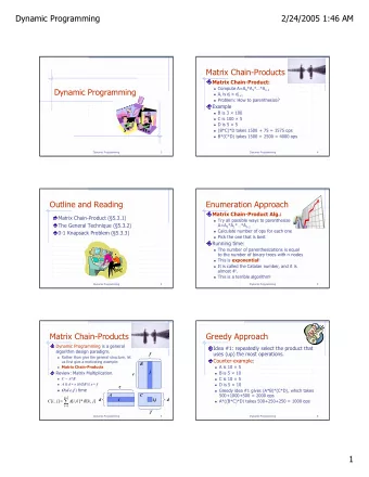
The Matrix-chain Multiplication Problem Problem: Matrix-Chain-Multiplication 1 Input: A sequence (chain) of n matrices A 1 , A 2 , A 3 , . . . , A n 2 Output: The product A 1 × A 2 × A 3 × · · · × A n Discussion: A i . columns = A i +1 . rows for every 1 ≤ i < n Assume A i has dimension p i − 1 × p i , for vector p [0 . . . n ] Matrix product is associative: ( A 1 × A 2 ) × A 3 = A 1 × ( A 2 × A 3 ) Exploit Associativity: Parenthesize A 1 × A 2 × A 3 × . . . A n so as to minimize the number of scalar multiplications (and thus the runtime) Dr. Christian Konrad Lecture 17/18: Matrix Chain Parenthesization 5 / 18

Order matters Example: Three matrices A 1 , A 2 , A 3 with dimensions A 1 : 10 × 100 A 2 : 100 × 5 A 3 : 5 × 50 ( p 0 = 10 , p 1 = 100 , p 2 = 5 , p 3 = 50) Computation of ( A 1 × A 2 ) × A 3 : A 1 × A 2 = A 12 requires 10 · 100 · 5 = 5000 multiplications A 12 × A 3 requires 10 · 5 · 50 = 2500 multiplications Total: 7500 multiplications Computation of A 1 × ( A 2 × A 3 ): A 2 × A 3 = A 23 requires 100 · 5 · 50 = 25000 multiplications A 1 × A 23 requires 10 · 100 · 50 = 50000 multiplications Total: 75000 multiplications Dr. Christian Konrad Lecture 17/18: Matrix Chain Parenthesization 6 / 18

The Matrix-Chain-Parenthesization Problem Problem: Matrix-Chain-Parenthesization 1 Input: A sequence (chain) of n matrices A 1 , A 2 , A 3 , . . . , A n 2 Output: A parenthesization of A 1 × A 2 × A 3 × · · · × A n that minimizes the number of scalar multiplications How many Parenthesizations P ( n ) are there? We write: A ij for the product A i × A i +1 × · · · × A j There is a final matrix multiplication: A 1 k × A ( k +1) n , for some 1 ≤ k ≤ n − 1. Hence: � 1 if n = 1 , P ( n ) = � n − 1 k =1 P ( k ) P ( n − k ) if n ≥ 2 . Example: Four matrices A 1 , A 2 , A 3 , A 4 A 1 × A 24 A 12 × A 34 A 13 × A 4 Dr. Christian Konrad Lecture 17/18: Matrix Chain Parenthesization 7 / 18

Number of Parenthesizations Example (continued): Four matrices A 1 , A 2 , A 3 , A 4 A 1 × A 24 A 12 × A 34 A 13 × A 4 2 � P (3) = P ( k ) P ( n − k ) = P (1) P (2) + P (2) P (1) = 2 k =1 3 � P (4) = P ( k ) P ( n − k ) = P (1) P (3) + P (2) P (2) + P (3) P (1) k =1 = P (3) + 1 + P (3) = 2 P (3) + 1 = 5 . 1 A 1 × (( A 2 × A 3 ) × A 4 ) 2 A 1 × (( A 2 × ( A 3 × A 4 )) 3 ( A 1 × A 2 ) × ( A 3 × A 4 ) 4 (( A 1 × A 2 ) × A 3 ) × A 4 5 ( A 1 × ( A 2 × A 3 )) × A 4 Dr. Christian Konrad Lecture 17/18: Matrix Chain Parenthesization 8 / 18

Number of Parenthesizations (2) A Bound on the Number of Parenthesizations: � 1 if n = 1 , P ( n ) = � n − 1 k =1 P ( k ) P ( n − k ) if n ≥ 2 . 1 , 1 , 2 , 5 , 14 , 42 , 132 , 429 , 1430 , 4862 , 16796 , 58786 , 208012 , 742900 , . . . It can be seen that there are Ω(2 n ) possibilities An efficient algorithm thus cannot try out all possibilities We will give a dynamic programming algorithm Dr. Christian Konrad Lecture 17/18: Matrix Chain Parenthesization 9 / 18

Optimal Substructure Optimal Substructure We say that a problem P exhibits optimal substructure if: An optimal solution to P contains within it optimal solutions to subproblems of P . Optimal Substructure in Matrix-Chain-Parenthesization Consider optimal solution to instance of size n Suppose that last product is A 1 k × A ( k +1) n Then the optimal solution contains optimal parenthesizations of A 1 × A 2 × · · · × A k and A k +1 × A k +2 × . . . A n Proof. Suppose it did not contain optimal parenthesizations of A 1 × A 2 × · · · × A k and of A k +1 × A k +2 × . . . A n . Then picking optimal parenthesizations of the two subproblems would give better solution to initial instance. Dr. Christian Konrad Lecture 17/18: Matrix Chain Parenthesization 10 / 18

Recursive Solution Optimal Solution to Subproblem: m [ i , j ] : minimum number of scalar multiplications needed to compute A i × A i +1 × · · · × A j = A ij Observe that m [ i , i ] = 0 (chain consists of single matrix A i ) Suppose j > i . Suppose last multiplication in optimal solution is: A ik × A ( k +1) j , for some k Then: cost of multiplying A ik × A ( k +1) j m [ i , j ] = m [ i , k ] + m [ k + 1 , j ] + p i − 1 p k p j ( A ik : p i − 1 × p k matrix, A ( k +1) j : p k × p j matrix) Since we do not know k , we try out all possibilities and choose the best solution: � 0 if i = j , m [ i , j ] = min i ≤ k < j { m [ i , k ] + m [ k + 1 , j ] + p i − 1 p k p j } if i < j . Dr. Christian Konrad Lecture 17/18: Matrix Chain Parenthesization 11 / 18

Computing the Optimal Costs � 0 if i = j , m [ i , j ] = min i ≤ k < j { m [ i , k ] + m [ k + 1 , j ] + p i − 1 p k p j } if i < j . Algorithmic Considerations: As in Pole-Cutting , we could implement this recursive formula directly. → exponential runtime Instead, we compute the table m [ i , j ] bottom up Observe that there are less than n 2 subproblems m [ i , j ] ( i and j take values in { 1 , . . . , n } ) We will see that computing one value m [ i , j ] takes O ( n ) time This yields an O ( n 3 ) time algorithm Dr. Christian Konrad Lecture 17/18: Matrix Chain Parenthesization 12 / 18

Dynamic Programming Algorithm Require: Integer n , vector of dimensions of matrices p so that matrix A i has dimensions p i − 1 × p i Let m [1 . . . n , 1 . . . n ] be a new array for i ← 1 . . . n do m [ i , i ] ← 0 for l ← 2 . . . n do { chain length } for i ← 1 . . . n − l + 1 do { left position } j ← i + l − 1 { right position } m [ i , j ] ← ∞ for k ← i . . . j − 1 do m [ i , j ] ← min { m [ i , j ] , m [ i , k ] + m [ k + 1 , j ] + p i − 1 p k p j } return m Algorithm Matrix-Chain-Value ( n , p ) � n − l +1 � i + l − 2 Runtime: O ( n 3 ) (by evaluating � n O (1)) l =2 i =1 k =1 Dr. Christian Konrad Lecture 17/18: Matrix Chain Parenthesization 13 / 18

Runtime Evaluation Useful Formula: b � 1 = b − a + 1 i = a n n − l +1 i + l − 2 n n − l +1 i + l − 2 � � � � � � O (1) = O (1) · 1 l =2 i =1 k =1 l =2 i =1 k =1 n n n n n n n � � � � � � � ≤ O (1) · 1 = O (1) · n = O (1) · n 1 l =1 i =1 k =1 l =1 i =1 l =1 i =1 n n 1 = O (1) · n 2 · n = O (1) n 3 � n = O (1) · n 2 � = O (1) · n l =1 l =1 O ( n 3 ) . = Dr. Christian Konrad Lecture 17/18: Matrix Chain Parenthesization 14 / 18

Example n = 4 and p = 3 7 6 2 9 1 2 3 4 1 2 3 4 for i ← 1 . . . n do m [ i , i ] ← 0 Dr. Christian Konrad Lecture 17/18: Matrix Chain Parenthesization 15 / 18

Example n = 4 and p = 3 7 6 2 9 1 2 3 4 1 0 2 0 3 0 4 0 for i ← 1 . . . n do m [ i , i ] ← 0 Dr. Christian Konrad Lecture 17/18: Matrix Chain Parenthesization 15 / 18

Example n = 4 and p = 3 7 6 2 9 1 2 3 4 1 0 2 0 3 0 4 0 for l ← 2 . . . n do for i ← 1 . . . n − l + 1 do j ← i + l − 1 { right position } m [ i , j ] ← ∞ for k ← i . . . j − 1 do m [ i , j ] ← min { m [ i , j ] , m [ i , k ] + m [ k + 1 , j ] + p i − 1 p k p j } l = 2 , i = 1 , j = 2 Dr. Christian Konrad Lecture 17/18: Matrix Chain Parenthesization 15 / 18

Example n = 4 and p = 3 7 6 2 9 1 2 3 4 1 0 2 126 0 3 0 4 0 for l ← 2 . . . n do for i ← 1 . . . n − l + 1 do j ← i + l − 1 { right position } m [ i , j ] ← ∞ for k ← i . . . j − 1 do m [ i , j ] ← min { m [ i , j ] , m [ i , k ] + m [ k + 1 , j ] + p i − 1 p k p j } l = 2 , i = 1 , j = 2 m [1 , 2] = m [1 , 1] + m [2 , 2] + p 0 p 1 p 2 = 0 + 0 + 3 · 7 · 6 = 126 Dr. Christian Konrad Lecture 17/18: Matrix Chain Parenthesization 15 / 18