
Matrix-Chain Multiplication Given : chain of matrices ( A 1 , A 2 , . - PowerPoint PPT Presentation
Matrix-Chain Multiplication Given : chain of matrices ( A 1 , A 2 , . . . A n ) , with A i having dimension ( p i 1 p i ) . Goal: compute product A 1 A 2 A n as quickly as possible Dynamic Programming 1 Multiplication of (
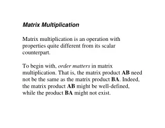
Matrix-Chain Multiplication Given : “chain” of matrices ( A 1 , A 2 , . . . A n ) , with A i having dimension ( p i − 1 × p i ) . Goal: compute product A 1 · A 2 · · · A n as quickly as possible Dynamic Programming 1
Multiplication of ( p × q ) and ( q × r ) matrices takes pqr steps Hence, time to multiply two matrices depends on dimensions! Example: : n = 4 . Possible orders: ( A 1 ( A 2 ( A 3 A 4 ))) ( A 1 (( A 2 A 3 ) A 4 )) (( A 1 A 2 )( A 3 A 4 )) (( A 1 ( A 2 A 3 )) A 4 ) ((( A 1 A 2 ) A 3 ) A 4 ) Suppose A 1 is 10 × 100 , A 2 is 100 × 5 , A 3 is 5 × 50 , and A 4 is 50 × 10 Order 2: 100 · 5 · 50 + 100 · 50 · 10 + 10 · 100 · 10 = 85 , 000 Order 5: 10 · 100 · 5 + 10 · 5 · 50 + 10 · 50 · 10 = 12 , 500 But: the number of possible orders is exponential! Dynamic Programming 2
We want to find Dynamic programming approach to optimally solve this problem The four basic steps when designing DP algorithm: 1. Characterize structure of optimal solution 2. Recursively define value of an optimal solution 3. Compute value of optimal solution in bottom-up fashion 4. Construct optimal solution from computed information Dynamic Programming 3
1. Characterizing structure Let A i,j = A i · · · A j for i ≤ j . If i < j , then any solution of A i,j must split product at some k , i ≤ k < j , i.e., compute A i,k , A k +1 ,j , and then A i,k · A k +1 ,j . Hence, for some k , cost is • cost of computing A i,k plus • cost of computing A k +1 ,j plus • cost of multiplying A i,k and A k +1 ,j .
Optimal (sub)structure: • Suppose that optimal parenthesization of A i,j splits between A k and A k +1 . • Then, parenthesizations of A i,k and A k +1 ,j must be optimal, too (otherwise, enhance overall solution — subproblems are indepen- dent!). • Construct optimal solution: 1. split into subproblems (using optimal split!), 2. parenthesize them optimally, 3. combine optimal subproblem solutions. Dynamic Programming 5
2. Recursively def. value of opt. solution Let m [ i, j ] denote minimum number of scalar multiplications needed to compute A i,j = A i · A i +1 · · · A j (full problem: m [1 , n ] ). Recursive definition of m [ i, j ] : • if i = j , then m [ i, j ] = m [ i, i ] = 0 ( A i,i = A i , no mult. needed). • if i < j , assume optimal split at k , i ≤ k < j . A i,k is p i − 1 × p k and A k +1 ,j is p k × p j , hence m [ i, j ] = m [ i, k ] + m [ k + 1 , j ] + p i − 1 · p k · p j . • We do not know optimal value of k , hence 0 if i = j m [ i, j ] = min i ≤ k<j { m [ i, k ] + m [ k + 1 , j ] if i < j + p i − 1 · p k · p j } Dynamic Programming 6
We also keep track of optimal splits: s [ i, j ] = k ⇔ m [ i, j ] = m [ i, k ] + m [ k + 1 , j ] + p i − 1 · p k · p j Dynamic Programming 7
3. Computing optimal cost Want to compute m [1 , n ] , minimum cost for multiplying A 1 · A 2 · · · A n . Recursively, according to equation on last slide, would take Ω(2 n ) (subproblems are computed over and over again). However, if we compute in bottom-up fashion , we can reduce run- ning time to poly ( n ) . Equation shows that m [ i, j ] depends only on smaller subproblems: for k = 1 , . . . , j − 1 , • A i,k is product of k − i + 1 < j − i + 1 matrices, • A k +1 ,j is product of j − k < j − i + 1 matrices. Algorithm should fill table m using increasing lengths of chains. Dynamic Programming 8
The Algorithm 1: n ← length [ p ] − 1 2: for i ← 1 to n do m [ i, i ] ← 0 3: 4: end for 5: for ℓ ← 2 to n do for i ← 1 to n − ℓ + 1 do 6: j ← i + ℓ − 1 7: m [ i, j ] ← ∞ 8: for k ← i to j − 1 do 9: q ← m [ i, k ] + m [ k + 1 , j ] + p i − 1 · p k · p j 10: if q < m [ i, j ] then 11: m [ i, j ] ← q 12: s [ i, j ] ← k 13: end if 14: end for 15: end for 16: 17: end for Dynamic Programming 9
Example A 1 ( 30 × 35 ), A 2 ( 35 × 15 ), A 3 ( 15 × 5 ), A 4 ( 5 × 10 ), A 5 ( 10 × 20 ), A 6 ( 20 × 25 ) Recall: multiplying A ( p × q ) and B ( q × r ) takes p · q · r scalar multi- plications. i 1 2 3 4 5 6 6 0 5 0 4 0 j 3 0 2 0 1 0 Dynamic Programming 10
Example A 1 ( 30 × 35 ), A 2 ( 35 × 15 ), A 3 ( 15 × 5 ), A 4 ( 5 × 10 ), A 5 ( 10 × 20 ), A 6 ( 20 × 25 ) Recall: multiplying A ( p × q ) and B ( q × r ) takes p · q · r scalar multi- plications. i 1 2 3 4 5 6 6 15,125 10,500 5,375 3,500 5,000 0 5 11,875 7,125 2,500 1,000 0 4 9,375 4,375 750 0 j 3 7,875 2,625 0 2 15,750 0 1 0 Dynamic Programming 11
4. Constructing optimal solution Simple with array s [ i, j ] , gives us optimal split points. Complexity We have three nested loops: 1. ℓ , length, O ( n ) iterations 2. i , start, O ( n ) iterations 3. k , split point, O ( n ) iterations Body of loops: constant complexity. Total complexity: O ( n 3 ) Dynamic Programming 12
All-pairs-shortest-paths • Directed graph G = ( V, E ) , weight function w : E → I R, | V | = n • Weight of path p = ( v 1 , v 2 , . . . , v k ) is w ( p ) = � k − 1 i =1 w ( v i , v i +1 ) • Assume G contains no negative-weight cycles • Goal: create n × n matrix of shortest path distances δ ( u, v ) , u, v ∈ V • 1st idea: use single-source-shortest-path alg (i.e., Bellman-Ford); but it’s too slow, O ( n 4 ) on dense graph Dynamic Programming 13
Adjacency-matrix representation of graph: • n × n adjacency matrix W = ( w ij ) of edge weights • assume 0 if i = j w ij = weight of ( i, j ) if i � = j and ( i, j ) ∈ E if i � = j and ( i, j ) �∈ E ∞ In the following, we only want to compute lengths of shortest paths, not construct the paths. Dynamic Programming 14
Dynamic programming approach, four steps: 1. Structure of a shortest path: Subpaths of shortest paths are shortest paths. Lemma. Let p = ( v 1 , v 2 , . . . , v k ) be a shortest path from v 1 to v k , let p ij = ( v i , v i +1 , . . . , v j ) for 1 ≤ i ≤ j ≤ k be subpath from v i to v j . Then, p ij is shortest path from v i to v j . Proof. Decompose p into p ij p jk p 1 i v 1 ❀ v i ❀ v j ❀ v k . Then, w ( p ) = w ( p 1 i ) + w ( p ij ) + w ( p jk ) . Assume there is cheaper p ′ ij from v i to v j with w ( p ′ ij ) < w ( p ij ) . Then p ′ p jk p 1 i ij v 1 ❀ v i ❀ v j ❀ v k is path from v 1 to v k whose weight w ( p 1 i )+ w ( p ′ ij )+ w ( p jk ) is less than w ( p ) , a contradiction. Dynamic Programming 15
2. Recursive solution and 3. Compute opt. value (bottom-up) Let d ( m ) = weight of shortest path from i to j that uses at most m ij edges. � 0 if i = j d (0) = ij ∞ if i � = j � � d ( m ) d ( m − 1) = min + w kj ij ik k at most m−1 edges k’s j i at most m−1 edges We’re looking for δ ( i, j ) = d ( n − 1) = d ( n ) = d ( n +1) = · · · ij ij ij Dynamic Programming 16
Alg. is straightforward, running time is O ( n 4 ) ( n − 1 passes, each computing n 2 d ’s in Θ( n ) time) Unfortunately, no better than before. . . Approach is similar to matrix multiplication: k a ik · b kj , O ( n 3 ) operations C = A · B , n × n matrices, c ij = � Replacing “ + ” with “ min ” and “ · ” with “ + ” gives c ij = min k { a ik + b kj } , very similar to d ( m ) k { d ( m − 1) = min + w kj } ij ik Hence D ( m ) = D ( m − 1) “ × ” W. Dynamic Programming 17
Floyd-Warshall algorithm Also DP, but faster (factor log n ) Define c ( m ) = weight of a shortest path from i to j with intermediate ij vertices in { 1 , 2 , . . . , m } . Then δ ( i, j ) = c ( n ) ij Dynamic Programming 18
Compute c ( n ) in terms of smaller ones, c ( <n ) : ij ij c (0) = w ij ij � � c ( m ) c ( m − 1) , c ( m − 1) + c ( m − 1) = min ij ij im mj (m−1) (m−1) c c m im mj i j (m−1) c ij intermediate vertices in {1,...,m−1} Dynamic Programming 19
Difference from previous algorithm: needn’t check all possible in- termediate vertices. Shortest path simply either includes m or doesn’t. Pseudocode: for m ← 1 to n do for i ← 1 to n do for j ← 1 to n do if c ij > c im + c mj then c ij ← c im + c mj end if end for end for end for Superscripts dropped, start loop with c ij = c ( m − 1) , end with c ij = c ( m ) ij ij Time: Θ( n 3 ) , simple code Dynamic Programming 20
Best algorithm to date is O ( V 2 log V + V E ) for dense graphs ( | E | ≈ | V | 2 ) can get APSP (with Floyd- Note: Warshall) for same cost as getting SSSP (with Bellman-Ford)! ( Θ( V E ) = Θ( n 3 ) ) Dynamic Programming 21
Recommend


More recommend
Explore More Topics
Stay informed with curated content and fresh updates.