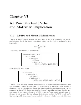
CS 140 : Matrix multiplication Warmup: Matrix times vector: - PowerPoint PPT Presentation
CS 140 : Matrix multiplication Warmup: Matrix times vector: communication volume Matrix multiplication I: parallel issues Matrix multiplication II: cache issues Thanks to Jim Demmel and Kathy Yelick (UCB) for some of these slides
CS 140 : Matrix multiplication • Warmup: Matrix times vector: communication volume • Matrix multiplication I: parallel issues • Matrix multiplication II: cache issues Thanks to Jim Demmel and Kathy Yelick (UCB) for some of these slides
Matrix-Matrix Multiplication (“DGEMM”) {implements C = C + A*B} for i = 1 to n for j = 1 to n for k = 1 to n C(i,j) = C(i,j) + A(i,k) * B(k,j) Work: 2*n 3 flops Memory: 3*n 2 words A(i,:) C(i,j) C(i,j) B(:,j) = + *
Parallel matrix multiply, C = C + A*B • Basic sequential algorithm: • C(i,j) += A(i,1) * B(1,j) + A(i,2) * B(1,j) + … + A(i,n) * B(n,j) • work = t 1 = 2n 3 floating point ops • Highly parallel: t p = 2n 3 / p is easy, for p up to at least n 2 • The issue is communication cost , as affected by: • Data layout • Structure & schedule of communication • Where’s the data?
Communication volume model • Network of p processors • Each with local memory • Message-passing • Communication volume (v) • Total size (words) of all messages passed during computation • Broadcasting one word costs volume p (actually, p-1) • No explicit accounting for communication time • Thus, we can ’ t model parallel efficiency or speedup; for that, we ’ d use the latency-bandwidth model (see extra slides)
Parallel Matrix Multiply with 1D Column Layout • Assume matrices are n x n and n is divisible by p (A reasonable assumption for analysis, not for code) p0 p1 p2 p3 p4 p5 p6 p7 • Let A(k) be the n-by-n/p block column that processor k owns • similarly B(k) and C(k) C(k) += A * B(k) • Now let B(i,k) be a subblock of B(k) with n/p rows C(k) += A(0) * B(0,k) + A(1) * B(1,k) + … + A(p-1) * B(p-1,k)
Matmul for 1D layout on a Processor Ring • Proc k communicates only with procs k-1 and k+1 • Different pairs of processors can communicate simultaneously • Round-Robin “ Merry-Go-Round ” algorithm Copy A(myproc) into MGR (MGR = “ Merry-Go-Round ” ) � C(myproc) = C(myproc) + MGR*B(myproc , myproc) � for j = 1 to p-1 � send MGR to processor myproc+1 mod p (but see deadlock below) � receive MGR from processor myproc-1 mod p (but see below) � C(myproc) = C(myproc) + MGR * B( myproc-j mod p , myproc) � � • Avoiding deadlock: � • even procs send then recv, odd procs recv then send � • or, use nonblocking sends and be careful with buffers � • Comm volume of one inner loop iteration = n 2 �
Matmul for 1D layout on a Processor Ring • One iteration: v = n 2 • All p-1 iterations: v = (p-1) * n 2 ~ pn 2 • Optimal for 1D data layout: • Perfect speedup for arithmetic • A(myproc) must meet each C(myproc) • “ Nice ” communication pattern – can probably overlap independent communications in the ring. • In latency/bandwidth model (see extra slides), parallel efficiency e = 1 - O(p/n)
MatMul with 2D Layout • Consider processors in 2D grid (physical or logical) • Processors can communicate with 4 nearest neighbors • Alternative pattern: broadcast along rows and columns p(0,0) p(0,1) p(0,2) p(0,0) p(0,1) p(0,2) p(0,0) p(0,1) p(0,2) = � * � p(1,0) p(1,1) p(1,2) p(1,0) p(1,1) p(1,2) p(1,0) p(1,1) p(1,2) p(2,0) p(2,1) p(2,2) p(2,0) p(2,1) p(2,2) p(2,0) p(2,1) p(2,2) • Assume p is square s x s grid
Cannon ’ s Algorithm: 2-D merry-go-round … C(i,j) = C(i,j) + Σ A(i,k)*B(k,j) k … assume s = sqrt(p) is an integer forall i=0 to s-1 … “ skew ” A left-circular-shift row i of A by i … so that A(i,j) overwritten by A(i,(j+i)mod s) forall i=0 to s-1 … “ skew ” B up-circular-shift B column i of B by i … so that B(i,j) overwritten by B((i+j)mod s), j) for k=0 to s-1 … sequential forall i=0 to s-1 and j=0 to s-1 … all processors in parallel C(i,j) = C(i,j) + A(i,j)*B(i,j) left-circular-shift each row of A by 1 up-circular-shift each row of B by 1
Cannon ’ s Matrix Multiplication C(1,2) = A(1,0) * B(0,2) + A(1,1) * B(1,2) + A(1,2) * B(2,2)
Initial Step to Skew Matrices in Cannon • Initial blocked input A(0,0) A(0,1) A(0,2) B(0,0) B(0,1) B(0,2) A(1,0) A(1,1) A(1,2) B(1,0) B(1,1) B(1,2) A(2,0) A(2,1) A(2,2) B(2,0) B(2,1) B(2,2) • After skewing before initial block multiplies A(0,0) A(0,1) A(0,2) B(0,0) B(1,1) B(2,2) A(1,1) A(1,2) A(1,0) B(1,0) B(2,1) B(0,2) A(2,2) A(2,0) A(2,1) B(2,0) B(0,1) B(1,2)
Skewing Steps in Cannon • First step A(0,0) A(0,1) A(0,2) B(0,0) B(1,1) B(2,2) A(1,1) A(1,2) A(1,0) B(1,0) B(2,1) B(0,2) A(2,2) A(2,0) A(2,1) B(2,0) B(0,1) B(1,2) • Second A(0,1) A(0,2) A(0,0) B(1,0) B(2,1) B(0,2) A(1,2) A(1,0) A(1,1) B(2,0) B(0,1) B(1,2) A(2,0) A(2,1) A(2,2) B(0,0) B(1,1) B(2,2) • Third A(0,2) A(0,0) A(0,1) B(2,0) B(0,1) B(1,2) A(1,0) A(1,1) A(1,2) B(0,0) B(1,1) B(2,2) B(1,0) B(2,1) B(0,2) A(2,1) A(2,2) A(2,0)
Communication Volume of Cannon ’ s Algorithm forall i=0 to s-1 … recall s = sqrt(p) left-circular-shift row i of A by i … v = n 2 / s for each i forall i=0 to s-1 up-circular-shift B column i of B by i … v = n 2 / s for each i for k=0 to s-1 forall i=0 to s-1 and j=0 to s-1 C(i,j) = C(i,j) + A(i,j)*B(i,j) left-circular-shift each row of A by 1 … v = n 2 for each k up-circular-shift each row of B by 1 … v = n 2 for each k ° Total comm v = 2*n 2 + 2 * s*n 2 ~ 2 * sqrt(p)*n 2 ° Computational intensity q = t 1 / v ~ n / sqrt(p) ° In latency/bandwidth model (see extra slides), parallel efficiency e = 1 - O(sqrt(p) / n)
Cannon is beautiful, but maybe too beautiful … • Drawbacks to Cannon: • Hard to generalize for p not a perfect square, A & B not square, dimensions not divisible by s = sqrt(p), different memory layouts, etc. • Memory hog – needs extra copies of local matrices. • Algorithm used instead in practice is SUMMA: • uses row and column broadcasts, not merry-go-round • see extra slides below for details • Comparing computational intensity = work / comm volume: • 1-D MGR has computational intensity q = O(n / p) • Cannon has computational intensity q = O(n / sqrt(p)) • SUMMA has computational intensity q = O(n / sqrt(p)log p)
Sequential Matrix Multiplication Simple mathematics, but getting good performance is complicated by memory hierarchy --- cache issues.
Naïve 3-loop matrix multiply {implements C = C + A*B} for i = 1 to n for j = 1 to n for k = 1 to n C(i,j) = C(i,j) + A(i,k) * B(k,j) Work: 2*n 3 flops Memory: 3*n 2 words A(i,:) C(i,j) C(i,j) B(:,j) = + *
3-Loop Matrix Multiply [Alpern et al., 1992] 12000 would take 1095 years 6 T = N 4.7 5 log cycles/flop 4 3 Size 2000 took 5 days 2 1 0 0 1 2 3 4 5 -1 log Problem Size O(N 3 ) performance would have constant cycles/flop Performance looks much closer to O(N 5 ) Slide source: Larry Carter, UCSD
3-Loop Matrix Multiply [Alpern et al., 1992] Page miss every iteration 6 5 log cycles/flop TLB miss every 4 iteration 3 Cache miss every 2 16 iterations Page miss every 512 iterations 1 0 0 1 2 3 4 5 log Problem Size Slide source: Larry Carter, UCSD
Avoiding data movement: Reuse and locality Conventional Storage Proc Proc Proc Hierarchy Cache Cache Cache L2 Cache L2 Cache L2 Cache interconnects potential L3 Cache L3 Cache L3 Cache Memory Memory Memory • Large memories are slow, fast memories are small • Parallel processors, collectively, have large, fast cache • the slow accesses to “ remote ” data we call “ communication ” • Algorithm should do most work on local data
Simplified model of hierarchical memory • Assume just 2 levels in the hierarchy, fast and slow • All data initially in slow memory • m = number of memory elements (words) moved between fast and slow memory • t m = time per slow memory operation • f = number of arithmetic operations • t f = time per arithmetic operation << t m • q = f / m ( computational intensity) flops per slow element access • Minimum possible time = f* t f when all data in fast memory • Actual time • f * t f + m * t m = f * t f * (1 + t m /t f * 1/q) • Larger q means time closer to minimum f * t f
“ Naïve ” Matrix Multiply {implements C = C + A*B} for i = 1 to n {read row i of A into fast memory} for j = 1 to n {read C(i,j) into fast memory} {read column j of B into fast memory} for k = 1 to n C(i,j) = C(i,j) + A(i,k) * B(k,j) {write C(i,j) back to slow memory} A(i,:) C(i,j) C(i,j) B(:,j) = + *
“ Naïve ” Matrix Multiply How many references to slow memory? m = n 3 read each column of B n times + n 2 read each row of A once + 2n 2 read and write each element of C once = n 3 + 3n 2 So q = f / m = 2n 3 / ( n 3 + 3n 2 ) ~= 2 for large n A(i,:) C(i,j) C(i,j) B(:,j) = + *
Blocked Matrix Multiply Consider A,B,C to be N by N matrices of b by b subblocks where b=n / N is called the block size for i = 1 to N for j = 1 to N {read block C(i,j) into fast memory} for k = 1 to N {read block A(i,k) into fast memory} {read block B(k,j) into fast memory} C(i,j) = C(i,j) + A(i,k) * B(k,j) {do a matrix multiply on blocks} {write block C(i,j) back to slow memory} A(i,k) C(i,j) C(i,j) = + * B(k,j)
Recommend
More recommend
Explore More Topics
Stay informed with curated content and fresh updates.
