DATA RECONCILIATION AND INSTRUMENTATION UPGRADE. OVERVIEW AND - PowerPoint PPT Presentation

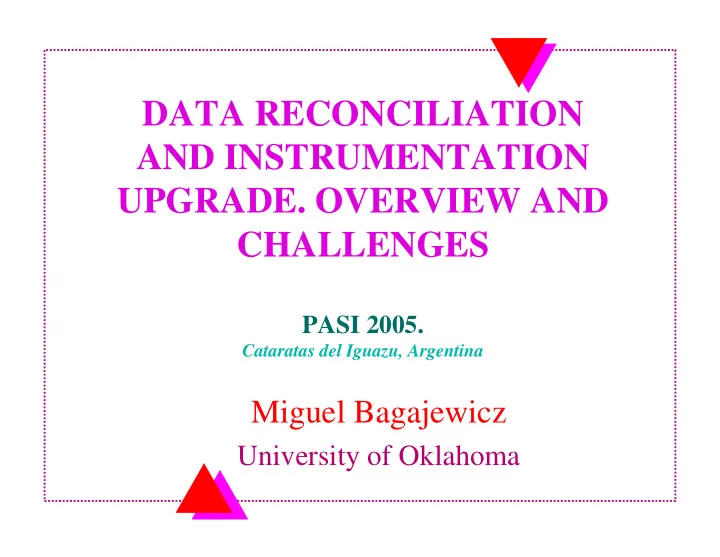
DATA RECONCILIATION AND INSTRUMENTATION UPGRADE. OVERVIEW AND CHALLENGES PASI 2005. Cataratas del Iguazu, Argentina Miguel Bagajewicz University of Oklahoma

OUTLINE • A LARGE NUMBER OF PEOPLE FROM ACADEMIA AND INDUSTRY HAVE CONTRIBUTED TO THE AREA OF DATA RECONCILIATION. • HUNDREDS OF ARTICLES AND THREE BOOKS HAVE BEEN WRITTEN. • MORE THAN 5 COMMERCIAL SOFTWARE EXIST. • ALTHOUGH A LITTLE YOUNGER, THE AREA OF INSTRUMENATION UPGRADE IS EQUALLY MATURE • ONE BOOK HAS BEEN WRITTEN

OUTLINE • OBSERVABILITY AND REDUNDANCY • DIFFERENT TYPES OF DATA RECONCILIATION - Steady State vs. Dynamic - Linear vs. Nonlinear • GROSS ERRORS - Biased instrumentation, model mismatch and outliers - Detection, identification and size estimation • INSTRUMENTATION UPGRADE • SOME EXISTING CHALLENGES • INDUSTRIAL PRACTICE

Simple Process Model of Mass Conservation f 2 f 4 f 8 f 10 U 1 U 4 f 1 f 6 f 7 U 3 U 2 U 5 f 3 f 5 f 9 f 11 f 1 - f 2 - f 3 = 0 f 2 - f 4 = 0 f 3 - f 5 = 0 f 4 + f 5 - f 6 = 0 f 6 - f 7 =0 Material Balance Equations f 7 - f 8 - f 9 = 0 f 8 - f 10 = 0 f 9 - f 11 = 0

Variable Classification f 2 f 4 f 8 f 10 U 1 U 4 f 1 f 6 f 7 U 3 U 2 U 5 f 3 f 5 f 9 f 11 Measured (M) Variables Observable (O) Unmeasured (UM) Unobservable (UO)

Variable Classification f 2 f 4 f 8 f 10 U 1 U 4 f 1 f 6 f 7 U 3 U 2 U 5 f 3 f 5 f 9 f 11 Redundant (R) Measured (M) Non-redundant (NR) Variables Observable (O) Unmeasured (UM) Unobservable (UO)

Conflict among Redundant Variables f 2 f 4 f 8 f 10 U 1 U 4 f 1 f 6 f 7 U 3 U 2 U 5 f 3 f 5 f 9 f 11 f 1 - f 7 =0 Material Balance Equations f 1 – f 8 – f 11 = 0

Conflict Resolution ~ ~ + − + − − T 1 Min f f Q f f [ ] [ ] R R R R R Data reconciliation in s.t. its simplest form ~ = E R f 0 R [ ] ( ) ~ − 1 = − + T T Analytical Solution f I Q E E Q E E f R R R R R R R R

Precision of Estimates = Γ z x If , and the variance of x is Q , then the variance ~ = Γ Γ of z is given by: T Q Q [ ] ( ) ( ) ~ − ~ − = − 1 1 = − + T T T T Q Q Q C C Q C C Q f I Q E E Q E E f R , F R , F R , F R R R , F R R R , F R R R R R R R R ~ + ~ = = f f Q Q NR , F NR , F NR NR ~ ~ ~ = + ~ ⎡ ⎤ f C f C f [ ] [ ] ~ Q = T ⎢ R ⎥ Q C C C C O RO R NRO NR O RO SRO RO SRO ⎣ ⎦ Q NR

Some Practical Difficulties • Variance-Covariance matrix is not Known • Process plants have a usually a large number of Tanks • Plants are not usually at Steady State • How many measurements is enough?

Estimation of the Variance- Covariance Matrix. ⎧ n ~ 1 ∑ = f f ⎪ R , i R , i k ⎪ n = k 1 ⎨ ( ) ( )( ) n ⎪ ~ ~ 1 ~ ~ ∑ = − − •Direct Approach Cov f , f f f f f ⎪ − R , i R , j R , i k R , i R , j k R , j ⎩ n 1 = k 1 •Indirect Approach + = = E f r T Cov ( r ) E Q E R R R R R Almasy and Mah (1984), Darouach et al., (1989) and 1) Obtain r Keller et al (1992) 2) Maximum likelihood estimate Q R However, this procedure is not good if outliers are present. Robust estimators have been proposed (Chen et al, 1997)

Tank Hold Up Measurements Level at t=t 0 Level at t=t 1 Pseudo-Stream Steady State formulations are used

The procedure is based on the following assumptions: ~ ~ + − + − − T 1 Min f f Q f f [ ] [ ] R R R R R a) A normal distribution of measurement errors. b) A single value per variable. ~ = E R f 0 c) A “steady-state” system. R a) Substantiated by the central limit theorem. 110 b) Also valid for means. 105 c) No plant is truly at “steady-state”. 100 Process oscillations occur. Therefore, it is said 95 90 that it is valid for a “pseudo-steady state” 1 250 Time system” 110 110 105 105 100 100 95 95 90 90 1 250 1 250 Time Time

Reconciliation of averages is equal to the average of reconciled values using dynamic data reconciliation (Bagajewicz and Jiang, 2000; Bagajewicz and Gonzales,2001). That is, there is no need to adjust the variance-covariance matrix for process variations.

Dynamic Data Reconciliation Linear Case(after cooptation): { } ~ ~ ∑ ~ ~ − + − − + + − + − − + T 1 T 1 Min [ f f ] Q [ f f ] [ V V ] Q [ V V ] Ri Ri Rf Ri Ri Ri Ri RV Ri Ri ∀ i ~ ~ d V = R B A f R dt ~ = C f 0 R When B=I, the Kalman filter can be used.

Dynamic Data Reconciliation { } ~ ~ ~ ~ ∑ + − + + − + − − + − − T 1 T 1 Min [ f f ] Q [ f f ] [ V V ] Q [ V V ] Ri Ri Rf Ri Ri Ri Ri RV Ri Ri ∀ i ~ ~ d V = R B A f R dt ~ = C f 0 R Difference Approach: Darouach, M. and M. Zasadzinski, 1991, Rollins, D. K. and S. Devanathan, 1993. ( ) ~ ~ ~ ~ − = = B V V A F C F 0 R , i R , i R , i R , i An algebraic system of equations follows. Integral Approach: Jiang and Bagajewicz, 1997. s α ∑ α R [ ] s s ∑ ∑ ≈ + − = ω + = R k k 1 R k 1 f t k B V V B t A t + R k + R R R 0 R k 1 R k 1 = = = k 0 k 0 k 0 The technique estimates the coefficients of polynomials.

Nonlinear Data Reconciliation N ∑ ~ ~ − − − T 1 Min [ x ( t ) z ] Q [ x ( t ) z ] M k M , k M k M , k = k 0 ~ d x ~ ~ = 1 g ( x , x ) 1 1 2 dt ~ ~ = g ( x , x ) 0 2 1 2 Applied in practice to steady state models with material, component and energy balances. In the dynamic case, orthogonal collocation was used (Liebmann et al, 1992) or linearization (Ramamurthi et al.,1993) or use of DAE (Albuquerque and Biegler, 1996).

Gross Errors

Types of Gross Errors 105 104 103 102 101 � Biases 100 99 98 97 96 � Leaks (Model departures) 95 1 250 Ti me � True outliers 104 103 102 Temperature 101 100 99 98 97 96 0 250 Time

Hypothesis Testing Global Test (Detection) ⎧ µ µ = T T ⎪ H : ( E Q E ) 0 0 R R R R R ⎨ ⎪ − µ µ ≠ γ = T 1 T T ⎩ r ( E Q E ) r H : ( E Q E ) 0 R R R 1 R R R R R − Distributi on : Chi Squared Nodal Test (Detection and Identification) ⎧ µ = ⎪ H : 0 0 r ⎨ r = i N 1 / 2 ⎪ µ ≠ Z n ⎩ H : 0 i T ( E Q E ) 1 r R R R ii Distributi on : Normal Maximum Power versions of this test were also developed. Rollins et al (1996) proposed an intelligent combination of nodes technique

Hypothesis Testing Principal Component (Tong and Crowe, 1995) T W : matrix of eigenvecto rs of ( E Q E ) r R R R Λ T : matrix of eigenvalue s of ( E Q E ) r R R R ⎧ µ = T ⎪ H : W 0 0 r ⎨ r = T p W r p r ~ N ( 0 , I ) ⎪ µ ≠ T ⎩ H : W 0 1 r Distributi on : Normal

Hypothesis Testing Measurement Test ⎧ φ − = ⎪ H : f 0 ~ + − 0 i i ⎨ f f = LCT i i Z ⎪ φ − ≠ χ ~ ⎩ H : f 0 ( Q ) 1 i i R ii Distributi on : Normal This test is inadmissible. Under deterministic conditions it may point to the wrong location.

Hypothesis Testing Generalized Likelihood ratio ⎧ µ = ⎪ H : 0 { } 0 r ⎨ Pr r H ⎪ µ = ⎩ H : bAe λ = 1 { } sup 1 r i Pr r H ∀ − i Distributi on : Chi Squared 0 − − − − T T 1 exp{ 0 . 5 ( r bAe ) ( E QE ) ( r bAe )} λ = i R R i sup − − T T 1 exp{ 0 . 5 r ( E QE ) r } ∀ b , i R R Leaks can also be tested.

Multiple Error Detection Serial Elimination Apply recursively the test and eliminate the measurement Serial Compensation Apply recursively the test, determine the size of the gross error and adjust the measurement Serial Collective Compensation Apply recursively the test, determine the sizes of all gross error and adjust the measurements

Multiple Error Detection Unbiased Estimation One shot collective information of all possible errors followed by hypothesis testing. Bagajewicz and Jiang, 2000, proposed an MILP strategy based on this. Two distributions approach Assume that gross error have a distribution with larger variance and use maximum likelihood methods (Romagnoli et al., 1981) (Tjoa and Biegler, 1991) (Ragot et al., 1992) Multiscale Bayesian approach. Bakshi et al (2001).

EQUIVALENCY THEORY � EXACT LOCATION DETERMINATION IS NOT ALWAYS POSSIBLE, REGARDLESS OF THE METHOD USED. � MANY SETS OF GROSS ERRORS ARE EQUIVALENT, THAT IS, THEY HAVE THE SAME EFFECT IN DATA RECONCILIATION WHEN THEY ARE COMPENSATED.

BASIC EQUIVALENCIES In a single unit a bias in an inlet stream is equivalent to a bias in an output stream. S1 S2 S 1 S 2 Measurement 4 3 Case 1 Reconciled data 3 3 Estimated bias 1 Case 2 Reconciled data 4 4 Estimated bias -1

BASIC EQUIVALENCIES In a single unit a bias in a stream is equivalent to a leak S1 S2 Leak S 1 S 2 Leak Measurement 4 3 Case1 Reconciled data 4 3 Estimated bias/leak 1 Case2 Reconciled data 4 4 Estimated bias/leak -1