Data assimilation and Markov Chain Monte Carlo techniques Moritz - PowerPoint PPT Presentation

Transformations of random variables More tools in your toolbox for working with random variables: Transformation by function h : Y = h ( X ) 30

Transformations of random variables More tools in your toolbox for working with random variables: Transformation by function h : Y = h ( X ) Distribution: P ( Y ∈ A ) = P ( X ∈ h − 1 ( A )). 30

Transformations of random variables More tools in your toolbox for working with random variables: Transformation by function h : Y = h ( X ) Distribution: P ( Y ∈ A ) = P ( X ∈ h − 1 ( A )). Simulation: Generate X , apply h . 30

Example: Sum of the eyes of two dice For example, consider two independent throws of six sided dies. 31

Sums and products of random variables In some cases the distribution of sums and products of random variables is known in closed form. Examples: Sum of jointly normal random variables is normal. Ratio of independent centred normal X and root of chi-squared V is t -distributed. 32

Example: Differential equation with uncertain parameter Example: Deterministic modelling + uncertainty. Differential equation d u ( t ) = − Θ u ( t ) d t 33

Example: Differential equation with uncertain parameter Example: Deterministic modelling + uncertainty. Differential equation d u ( t ) = − Θ u ( t ) d t with uncertainty about the parameter Θ and starting value u (0) = U , quantified by U ∼ N (5 , 3) Θ ∼ N (0 . 5 , 0 . 1) . 33

Example: Differential equation Model is of functional form u ( t ) = f t (Θ , U ) with f t ( θ, u ) = exp( − θ t ) u the solution of the ODE. 34

Example: Differential equation Model is of functional form u ( t ) = f t (Θ , U ) with f t ( θ, u ) = exp( − θ t ) u the solution of the ODE. Explore model through simulations https: //nextjournal.com/mschauer/probabilistic-programming 34

Exact computations Example: Sum of uniform random variables Z = X 1 + X 2 , where X 1 , X 2 ∼ U [0 , 1] independent. 35

Exact computations Example: Sum of uniform random variables Z = X 1 + X 2 , where X 1 , X 2 ∼ U [0 , 1] independent. Z has triangular distribution with density � x 0 ≤ x ≤ 1 f Z ( x ) = 2 − x 1 ≤ x ≤ 2 . 35

Working with mean and variance Sometimes it is sufficient to determine mean and variance of the result of operations on random variables. For sums of r.v. X and Y : E [ X + Y ] = E X + E Y . Var( aX + Y ) = a 2 Var( X ) + Var( Y ) if X , Y independent 36

Working with mean and variance Sometimes it is sufficient to determine mean and variance of the result of operations on random variables. For sums of r.v. X and Y : E [ X + Y ] = E X + E Y . Var( aX + Y ) = a 2 Var( X ) + Var( Y ) if X , Y independent In the situation of the central limit theorem, a sum of random variables can approximated by a normal with the right mean and variance. 36

Error propagation Independent X 1 . . . X n random with mean 10 and std. deviation √ 0 . 09. Z = � n 0 . 3 = i =1 X i . Z is approx. N (10 n , 0 . 09 n ) distributed ± 0 . 3 √ n Z = 10 n ���� � �� � mean std . dev 37

Error propagation Independent X 1 . . . X n random with mean 10 and std. deviation √ 0 . 09. Z = � n 0 . 3 = i =1 X i . Z is approx. N (10 n , 0 . 09 n ) distributed ± 0 . 3 √ n Z = 10 n ���� � �� � mean std . dev Very different from how the engineer argues: X 1 , . . . , X n are quantities approximately in the interval [9 . 7 , 10 . 3] Z ∈ [9 . 7 n , 10 . 3 n ] or Z = 10 n ± 0 . 3 n . 37

Julia programming language I have prepared some things using the programming language Julia. You can follow the course and lab using a programming language you are familar with, but you might enjoy giving Julia a try. There are many online ressources at julialang.org/learning/ . 38

Setup • Install Julia. Download the Julia 1.1 for your operating system from julialang.org or • Make a free account on https://nextjournal.com/ . Nextjournal is an online notebook environment running Julia (you need a working internet connection to use it.) • In any case, download https: //www.dropbox.com/s/yvwgz71zgvkj7sg/icecoredata.csv and read https://nextjournal.com/mschauer/bayesian-filter for the lab. 39

Markov chain

Simple Markov chain Recursively, let X i = h ( X i − 1 , Z i ) , i > 0 and X 0 ∼ g using independent identically distributed innovation or noise random variables Z 1 , . . . , Z n , . . . . 40

Example: Autoregressive chain Autoregressive chain: Take η ∈ (0 , 1), h ( x , z ) = η x + z and i . i . d . Z 1 , . . . , Z n , ∼ N (0 , 1) . So X i = η X i − 1 + Z i , i > 0 . 41

Example: Autoregressive chain Then Var( X i ) = Var( η X i − 1 + Z i ) = η 2 Var( X i − 1 ) + 1 . 42

Example: Autoregressive chain Then Var( X i ) = Var( η X i − 1 + Z i ) = η 2 Var( X i − 1 ) + 1 . Assume that X 0 is normal with mean zero. Then all X i are equally normal with mean zero. Setting Var( X i ) ≡ σ 2 42

Example: Autoregressive chain Then Var( X i ) = Var( η X i − 1 + Z i ) = η 2 Var( X i − 1 ) + 1 . Assume that X 0 is normal with mean zero. Then all X i are equally normal with mean zero. Setting Var( X i ) ≡ σ 2 and solving σ 2 = η 2 σ 2 + 1 gives 1 σ 2 = 1 − η 2 . { X 1 , X 2 , . . . } is a Markov chain with stationary distribution 1 X i ∼ N (0 , 1 − η 2 ) . 42

Filtering

Smoothing/Filtering Start with joint density factorized as f ( x , y ) = f ( y | x ) f ( x ) This is convenient if e.g. x is a parameter with prior and the density of Y given X = x is determined by the model. Y is observed. 43

Smoothing/Filtering Start with joint density factorized as f ( x , y ) = f ( y | x ) f ( x ) This is convenient if e.g. x is a parameter with prior and the density of Y given X = x is determined by the model. Y is observed. Then as before f ( y | x ) f ( x ) f ( x , y ) f ( x | y ) = f ( y | x ′ ) f ( x ′ ) d x ′ = f ( x ′ , y ) d x ′ . � � 43

Random walk filter example for the lab See https://nextjournal.com/mschauer/bayesian-filter for example and details. 44

Random walk filter example for the lab The North Greenland Ice Core Project obtained a core sample of ice from drilling through the arctic ice shield. Scientists are interested in a quantity X t (the past δ 18 O values) which changes over time, written as t = 1 , . . . , n . 45

Measurements They have produced a sequence of n measurements Y 1 , . . . , Y n and, as the measurement errors stem from a variety of unrelated causes, model the measurement errors ǫ t at time t , Y t = X t + ǫ t . as independent random variables ǫ t with Gaussian distribution N (0 , σ 2 ) with variance σ 2 for each t = 1 , . . . , n . 46

Model Model X t +1 = X t + η t , for t = 1 , . . . , n − 1, where η t are independent normally distributed N (0 , s 2 ) with mean zero and variance s 2 for t = 1 , . . . , n . 47

Filter The filtered distribution of X t is the conditional distribution of X t at time t given observations Y 1 = y 1 , Y 2 = y 2 up to and including Y t = y t . It captures what we know about X t if we have seen the measurement points y 1 , y 2 , . . . , y t . 48

Kalman filtering equations For a random walk model with independent observation errors as above the filtered distribution of X t is a normal distribution and its mean µ t and variance p 2 t can be computed recursively using the filtering equations p 2 t = σ 2 K t µ t = µ t − 1 + K t ( y t − µ t − 1 ) with K t the so called Kalman gain s 2 + p 2 t − 1 K t = t − 1 + σ 2 , t > 1 s 2 + p 2 p 2 and K 1 = 0 + σ 2 . 0 p 2 49

Kalman filtering equations The mean of the filtered distribution, µ t , serves as estimate of the unknown location of X t and the standard deviation p t can be seen as measure of uncertainty about the location. 50

Full Kalman filter The more general Kalman filter for multivariate linear models x k = Φ x k 1 + b + w k , w k ∼ N (0 , Q ) y k = Hx k + v k , v k ∼ N (0 , R ) proceeds similarly. 51

Hierarchical Bayesian modelling

Outline • Hierarchical probabilistic model • Bayesian inference • Monte Carlo methods • Metropolis–Hastings 52

Hierarchical models Use hierarchical models to deal with • dependency between variables • indirect observations and missing data • smoothing/filtering • Generally: If the data generating process is somewhat understood 53

A dilemma when modelling groups Pool all groups together. Model each group separately. • Small sample sizes problematic. • Ignore latent differences. • Many more parameters to • Observations are not estimate. independent. • Ignores latent similarity. Hierarchical modelling shows a way out... 54

Example: Group means model Latent group means b i ∼ N ( µ, σ 2 b ) with density φ i for m groups. Specimen j from group i y ij ∼ N ( b i , σ 2 y ) with density φ ij ( · − b i ). Factorisation of the joint density � � φ i ( b i ) φ ij ( y ij − b i ) i ∈ I j ∈ J i 55

Example: Group means model Latent group means b i ∼ N ( µ, σ 2 b ) with density φ i for m groups. Specimen j from group i y ij ∼ N ( b i , σ 2 y ) with density φ ij ( · − b i ). Factorisation of the joint density � � φ i ( b i ) φ ij ( y ij − b i ) i ∈ I j ∈ J i Only the specimens are observed, the conditional density is � � � p ( y ij ) ( b 1 , . . . , b m ) = φ i ( b i ) φ ij ( y ij − b i ) d b 1 · · · d b m i ∈ I j ∈ J i 55

Bayesian net This is an example of a Bayesian net. The variables with nodes together with the parent operator pa form a DAG, a directed, acyclic graph. In general, the joint density in a Bayesian net can be factorises in the form n � p ( x 1 , . . . , x n ) = p ( x i | pa( x i )) i =1 56

Bayesian net, factor graph representation � p ( x 1 , . . . , x d ) = f α ( x α ) α ∈ F where α ⊂ { 1 , . . . , d } and x α is the tuple of variables ( x i ) i ∈ α . 57

Bayes’ formula for hierarchical models 58

Markov Chain Monte Carlo

What is on the menu • Markov chain Monte Carlo methods. Computational algorithms for generating samples from a probability distribution say with density x �→ p ( x ) for example a posterior density in Bayesian statistics. • The Metropolis-Hastings algorithm, from which many MCMC methods can be derived. 59

Recap: Markov chain A Markov chain • is a sequence of random variables X 1 , X 2 , . . . (with values in some state space E ) • with the Markov property: P ( X i ∈ B | X i − 1 = x i − 1 , . . . , X 1 = x 1 ) = P ( X i ∈ B | X i − 1 = x i − 1 ) . 60

Recap: Markov chain A Markov chain • is a sequence of random variables X 1 , X 2 , . . . (with values in some state space E ) • with the Markov property: P ( X i ∈ B | X i − 1 = x i − 1 , . . . , X 1 = x 1 ) = P ( X i ∈ B | X i − 1 = x i − 1 ) . The transition kernel Q ( x ; B ) = P ( X i ∈ B | X i − 1 = x ) of a time-homogenous Markov chain fully describes the evolution of the chain. Denote its density in x ′ by q ( x ; x ′ ) . 60

Markov chain Monte Carlo Generate Markov chain X 1 , X 2 , . . . with equilibrium density p . Under the conditions of the ergodic theorem still n � 1 � a . s . f ( X i ) − − → f ( x ) p ( x ) d x , n i =1 but the convergence becomes slower. 61

Bayesian inference A typical application of MCMC is in Bayesian inference. Posterior density π ( · | y ) is proportional to p θ ( y ) π ( θ ) . ( y is an observation with density p θ ( y ) and π is a prior distribution of a parameter θ ) Statistical questions should have answers of the form � f ( θ ) d π ( θ | y ) . 62

Expectations Statistical questions should have answers of the form � f ( θ ) d π ( θ | y ) . For example posterior mean and variance or probabilities arise this way. “Statistical” questions which cannot be posed as expectations of the posterior are very problematic. What would be interesting choices of f ? 63

Expectations Statistical questions should have answers of the form � f ( θ ) d π ( θ | y ) . For example posterior mean and variance or probabilities arise this way. “Statistical” questions which cannot be posed as expectations of the posterior are very problematic. What would be interesting choices of f ? Probabilities are expectations of indicators and the median is minimiser of expected deviation. 63

Probabilistic programming Hierarchical Bayesian model s 2 ∼ InverseGamma(2 , 3) m ∼ N (0 , s 2 ) x ∼ N ( m , s 2 ) y ∼ N ( m , s 2 ) What is the posterior distribution of parameters s and m given observations x = 1 . 5, y = 2? 64

Probabilistic programming Short illustration using the Turing.jl package in . https://nextjournal.com/mschauer/probabilistic-programming 65

Probabilistic programming Generated Markov chain. 66

Probabilistic programming Posterior density estimates. 67

Markov chains and detailed balance The chain is in detailed balance if there is a density p such that p ( x ) q ( x ; x ′ ) = p ( x ′ ) q ( x ′ ; x ) , i.e. symmetry of the joint distribution of two iterates X , X ′ when starting the chain in X ∼ p . Implies that p is stationary density � p ( x ) q ( x ; x ′ ) d x ′ p ( x ) = � p ( x ′ ) q ( x ′ ; x ) d x ′ = . � �� � the density after one step (A sufficient condition.) 68

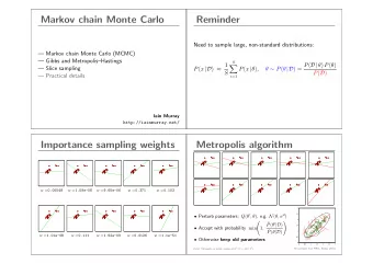
Metropolis-Hastings algorithm Starting point is a Markov chain with some transition density q ( x ; x ′ ) . For example, a symmetric random walk, q ( x ; x ′ ) = C exp( −� x − x ′ � 2 ) = q ( x ′ ; x ) . 2 σ 2 mh 69

How to obtain a chain with stationary density p Define a new chain, for which detailed balance holds for p by modifying the transition kernel. 70

Metropolis-Hastings algorithm Define the Metropolis-Hastings acceptance probability � p ( x ′ ) q ( x ′ ; x ) � α ( x ; x ′ ) = min p ( x ) q ( x ; x ′ ) , 1 . 71

Metropolis-Hastings algorithm Define the Metropolis-Hastings acceptance probability � p ( x ′ ) q ( x ′ ; x ) � α ( x ; x ′ ) = min p ( x ) q ( x ; x ′ ) , 1 . Starting from X 1 , we recursively... • Given X i , draw random proposal X ◦ i +1 from the density q ( X i ; · ) • With probability α ( X i ; X ◦ i +1 ) accept and move: X i +1 = X ◦ i +1 , else reject and stay: X i +1 = X i . 71

Detailed balance Proposition: This creates a Markov chain with a new Markov kernel Q MH ( x , · ) such that detailed balance holds for p . 72

Detailed balance Proposition: This creates a Markov chain with a new Markov kernel Q MH ( x , · ) such that detailed balance holds for p . That means hat the joint law p ( x ) Q MH ( x , d x ′ ) d x is symmetric: p ( x ) Q MH ( x ; d x ′ ) d x = p ( x ′ ) Q MH ( x ′ ; d x ) d x ′ . 72

Detailed balance Proposition: This creates a Markov chain with a new Markov kernel Q MH ( x , · ) such that detailed balance holds for p . That means hat the joint law p ( x ) Q MH ( x , d x ′ ) d x is symmetric: � � � � p ( x ) Q MH ( x ; d x ′ ) d x = p ( x ′ ) Q MH ( x ′ ; d x ) d x ′ ∀ A , B A B B A 72

Proof: � p ( x ′ ) q ( x ′ ; x ) � α ( x ; x ′ ) = min p ( x ) q ( x ; x ′ ) , 1 For any x , x ′ , at least one of α ( x ; x ′ ) , α ( x ′ ; x ) equals 1. 73

Proof: To show symmetry take x � = x ′ with α ( x ; x ′ ) < 1 (otherwise switch x , x ′ below.) Then p ( x ) Q MH ( x , d x ′ ) d x = p ( x ) q ( x ; x ′ ) α ( x ; x ′ ) d x d x ′ = p ( x ) q ( x ; x ′ ) p ( x ′ ) q ( x ′ ; x ) p ( x ) q ( x ; x ′ ) d x d x ′ 73