CSCE 488: Performance Evaluation Proper experimental technique is - PDF document
Why are We Here? CSCE 488: Performance Evaluation Proper experimental technique is essential to system verification Without it, were just hoping that everything works OK Stephen D. Scott Here Ill focus on timing verification,
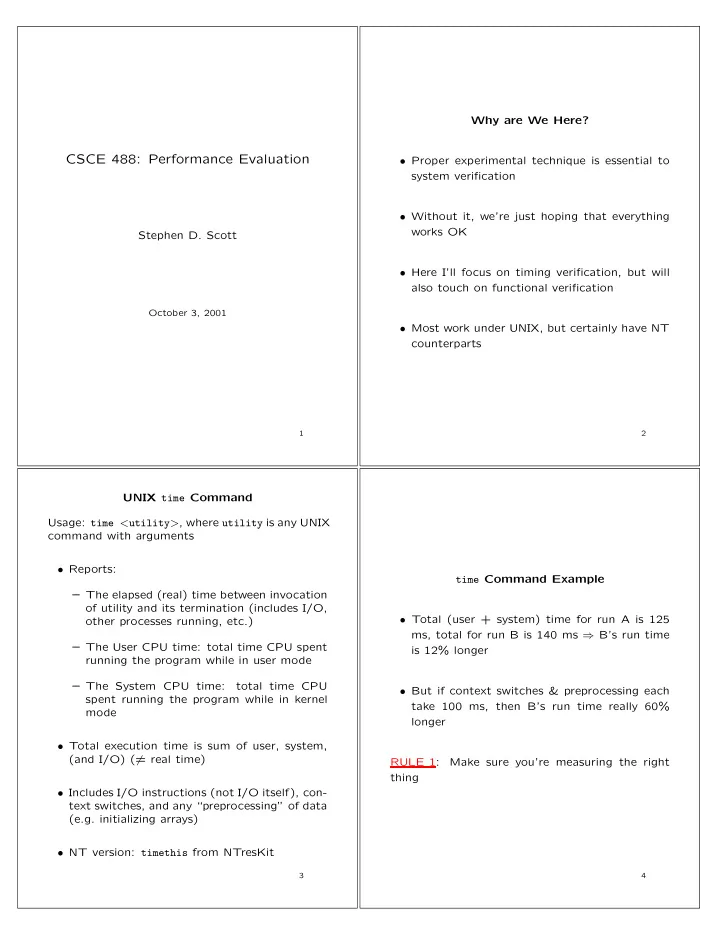
Why are We Here? CSCE 488: Performance Evaluation • Proper experimental technique is essential to system verification • Without it, we’re just hoping that everything works OK Stephen D. Scott • Here I’ll focus on timing verification, but will also touch on functional verification October 3, 2001 • Most work under UNIX, but certainly have NT counterparts 1 2 UNIX time Command Usage: time < utility > , where utility is any UNIX command with arguments • Reports: time Command Example – The elapsed (real) time between invocation of utility and its termination (includes I/O, • Total (user + system) time for run A is 125 other processes running, etc.) ms, total for run B is 140 ms ⇒ B’s run time – The User CPU time: total time CPU spent is 12% longer running the program while in user mode – The System CPU time: total time CPU • But if context switches & preprocessing each spent running the program while in kernel take 100 ms, then B’s run time really 60% mode longer • Total execution time is sum of user, system, (and I/O) ( � = real time) RULE 1: Make sure you’re measuring the right thing • Includes I/O instructions (not I/O itself), con- text switches, and any “preprocessing” of data (e.g. initializing arrays) • NT version: timethis from NTresKit 3 4
More Precise Timing Measurements ACE’s Profile Timer • Use system calls around blocks of code to grab • Developed by Doug Schmidt in his ACE (Adap- precise system timing info tive Communication Environment) package: http://www.cs.wustl.edu/~schmidt/ACE.html • Times measured from arbitrary point in past (e.g. reboot) in number of “clock ticks” • Timer is just a small part • Can use to get time stamps at different points in the code and compute difference • Gets up to (down to?) nanosecond precision (not nanosec. accuracy) E.g. #include <sys/types.h> #include <sys/times.h> • Requires sys/procfs.h (not in NT?) clock_t times(struct tms *buffer); where E.g. struct tms { main() clock_t tms_utime; /* user time of current proc. */ { clock_t tms_stime; /* system time of current proc. */ Profile_Timer timer; clock_t tms_cutime; /* child user time of current proc. */ Profile_Timer::Elapsed_Time et; clock_t tms_cstime; /* child sys. time of current proc. */ }; timer.start(); /* run code to be timed here */ timer.stop(); • Can also use clocks() (ANSI C) or times() timer.elapsed_time(et); /* compute elapsed time */ (SVr4, SVID, X/OPEN, BSD 4.3 and POSIX) cout << "time(in secs): " << et.user_time; } 6 5 Caveat Application of Timer Example: Merge Sort vs. Insertion Sort • Most system-independent timers are only up- dated every 10 ms • For sorting 20 items, IS took 2 . 0 × 10 − 5 sec, made 363 comparisons • Thus cannot rely on measurements more fine than that, even though they’re available • For sorting 20 items, MS took 5 . 8 × 10 − 5 sec, made 658 comparisons • One approach: run same routine multiple times and take average • Conclusion: IS is more than twice as fast as MS [FALLACY] – Can have problems with caches – Workaround: after every run, “flush” the RULE 2: Measure trends cache, or use new dataset each time 7 8
7000 "is-time" "ms-time" 6000 5000 OK, Tough Guy, Let’s Measure Trends 4000 • Choose already sorted inputs to test the algorithm [INCORRECT TREND] 3000 RULE 3: Take average over several inputs of the same size 2000 1000 0 1.6 1.4 1.2 1 0.8 0.6 0.4 0.2 0 10 9 7000 "is-sorted-time" "ms-sorted-time" 6000 Sampling Theory 5000 • What inputs should we use to test? • Ideally, what you would see in practice 4000 – Don’t always know this 3000 • Next best thing: all possible inputs (exponen- tially or infinitely big) or a (uniformly) ran- domly selected set 2000 • Rule of thumb: try at least 30 random sets 1000 and take mean 0 0.02 0.018 0.016 0.014 0.012 0.01 0.008 0.006 0.004 0.002 0 11 12
Sampling Theory (cont’d) Sampling Theory (cont’d) • Based on Central Limit Theorem, which states that regardless of the data’s distribution, ¯ X ’s dist. is approximately Gaussian (normal) with • Mean of X 1 , . . . , X m (e.g. sort times for m in- variance ≈ s/ √ m , assuming m large enough X = (1 /m ) � m ¯ puts, each of size n ): i =1 X i 0.4 0.4 �� m 0.35 0.35 i =1 ( X i − ¯ X ) 2 • Standard deviation s = 0.3 0.3 m − 1 0.25 0.25 0.2 0.2 � i =1 X i ) 2 0.15 0.15 �� m � m i =1 X 2 � − ( m 0.1 0.1 = i (compute on-line) 0.05 0.05 m ( m − 1) 0 0 -3 -2 -1 0 1 2 3 -3 -2 -1 0 1 2 3 N % of area (probability) lies in µ ± z N σ • If m ≥ 30, we are 95% confident that the true mean is approximately in N % 50% 68% 80% 90% 95% 98% 99% X ± z 0 . 025 ( s/ √ m ) = ¯ X ± 1 . 96( s/ √ m ) z N 0.67 1.00 1.28 1.64 1.96 2.33 2.58 ¯ (1) N % of area lies < µ + z ′ N σ or > µ − z ′ N σ , where and we are 95% confident that the true mean z ′ N = z 100 − (100 − N ) / 2 is approximately at most X + z 0 . 05 ( s/ √ m ) = ¯ X + 1 . 645( s/ √ m ) ¯ (2) N % 50% 68% 80% 90% 95% 98% 99% z ′ 0.0 0.47 0.84 1.28 1.64 2.05 2.33 N (1) is two-sided interval and (2) is one-sided Consult your Statistics text for more info, esp. on z α ’s 13 14 Functional Verification Hardware Timing • Hardware: CAD tools, e.g. Xilinx Foundation • Software: run directly or use source-level debugger • Several CAD tools (incl. Xilinx Foundation) will perform timing analysis of designs after mapped to implementation technology • For both, test boundary and nominal condi- tions; go for high % cover of code/data paths – Make sure you use the right technology! • When practicable, compare to hand simulation • An important aspect of this: critical path analysis, (e.g. with smaller inputs) where the longest input-to-output path (in terms of time) is estimated and timed, which bounds • HW/SW testing is active area of research (e.g. the maximum clock rate Prof. Elbaum) • Formal methods: one approach used for veri- • Don’t forget about e.g. printed circuit board fication of hw and sw designs, has been used delays, memory access latency, etc. on specific code sets/designs, not yet used in the large – Take max delay between hardware and soft- ware components • Extra problems occur with concurrency, e.g. multiple threads 15 16
Recommend
More recommend
Explore More Topics
Stay informed with curated content and fresh updates.


