CS485/685 Lecture 15: Feb 28, 2012 Probably Approximately Correct - PDF document

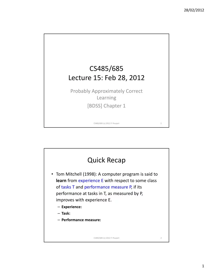
28/02/2012 CS485/685 Lecture 15: Feb 28, 2012 Probably Approximately Correct Learning [BDSS] Chapter 1 CS485/685 (c) 2012 P. Poupart 1 Quick Recap • Tom Mitchell (1998): A computer program is said to learn from experience E with respect to some class of tasks T and performance measure P, if its performance at tasks in T, as measured by P, improves with experience E. – Experience: – Task: – Performance measure: CS485/685 (c) 2012 P. Poupart 2 1

28/02/2012 Performance Measure • So far, we measured the performance of algorithms empirically – Train with training set and measure performance with a separate test set – K ‐ fold cross validation: • Can reuse the data for training and testing • Average performance over multiple splits of the data to improve statistical reliability • Open questions: – How much data do we need to learn a task? – When is a task learnable? CS485/685 (c) 2012 P. Poupart 3 Computational Complexity • Computational Complexity : branch of the theory of computation that focuses on classifying computational problems based on their inherent difficulty – Time complexity – Space complexity • In machine learning, we also consider – Data complexity (a.k.a. sample complexity) CS485/685 (c) 2012 P. Poupart 4 2

28/02/2012 Computational Complexity • Time/space complexity – How do time/space requirements vary with the size of the input? • Data complexity – How do data requirements (size of the input) vary with the performance level? • Problem: we can’t guarantee a performance level because the training data is usually different from the data that the algorithm will encounter in the future • Idea: study data requirements as a function of a probabilistic performance level CS485/685 (c) 2012 P. Poupart 5 Formal Model (Supervised Classification) 1. The learner’s input Domain set � (e.g., possible emails in spam filtering) a. Label set � (e.g., �����, ~����� ) b. For convenience assume that � � �0,1� or ��1,1� Training data � � � � � , � � , � � , � � , … , � � , � � � c. sequence of pairs in � � � 2. The learner’s output: hypothesis or prediction rule �: � → � e.g., decision tree, k ‐ NN rule, linear separator CS485/685 (c) 2012 P. Poupart 6 3

28/02/2012 Formal Model (Supervised Classification) 3. Data generation model training and testing data is sampled independently and identically (i.i.d.) from an unknown distribution �. � � , � � ~ � ∀� 4. Performance measure: probability of error � � � � � � �� � � �� � ∑ � � �, � ��� � � �� �,� true loss, but � is unknown CS485/685 (c) 2012 P. Poupart 7 Empirical Risk Minimization • � is unknown, but � is known � � � � ∑ � � � � � � � � � • Empirical risk minimization (ERM): Find � � that minimizes � � ��� • How good is ERM? – It can be pretty bad (due to overfitting) CS485/685 (c) 2012 P. Poupart 8 4

28/02/2012 Papaya example • Consider a papaya prediction problem CS485/685 (c) 2012 P. Poupart 9 Papaya example • Hypothesis � � : if a papaya is identical to a previously tasted papaya, predict the same taste. Otherwise, assume that it tastes bad. • Let � � � � �� � if ∃� such that � � � � 0 otherwise • Then � � � � � but � � � � � • This is an example of poor generalization (overfitting) CS485/685 (c) 2012 P. Poupart 10 5

28/02/2012 Generalization • How does the accuracy of � � vary with the amount of data? – As |�| ↑ , then |� � � � � � � | ↓ • How much data do we need to make sure that the hypothesis � � found by ERM is not much worse than the best hypothesis � ∗ most of the time? � � � ������ �∈� � � ��� � ∗ � ������ �∈� � � ��� CS485/685 (c) 2012 P. Poupart 11 Assumptions 1. Finite Hypothesis class Assume � is finite (and chosen before receiving �� – 2. Realizable assumption: there exists a perfect hypothesis � ∗ ∈ � i.e., ∃� ∗ ∈ � such that � � � ∗ � 0 – This implies that for any training set � , � � � ∗ � 0 – Since � ∗ is deterministic, this implies that � � ��|�� is – deterministic 3. i.i.d. assumption: Data is independently and identically distributed from � – CS485/685 (c) 2012 P. Poupart 12 6

28/02/2012 Analysis • Find sample size � � |�| such that � � � � � � – Here � is a bound on the true loss • Problem: since � is obtained by a random process, � � and � � �� � � are random. • Instead: find sample size � � |�| such that Pr � � � � � � � � – Here � is a bound on the probability that we obtain a sample � for which � � is bad (i.e., � � � � � � ) – Hence 1 � � is our confidence in the bound � CS485/685 (c) 2012 P. Poupart 13 Bound Corollary: Let � be finite, � ∈ �0,1� , � � 0 and � log � � � � then for any � (for which the realizable assumption holds), with probability at least 1 � � we have that � � � � � � CS485/685 (c) 2012 P. Poupart 14 7

28/02/2012 Proof Proof: we need to show that � �~� � � � � � � � � � • Let � � � �� ∈ �|� � � � �� be the set of bad hypotheses • By the realizable assumption, � � � � � 0 . • This implies that � � � � � � can only happen if for some � ∈ � � we have � � � � 0 . • Hence �|� � � � � � ⊆ ��|∃� ∈ � � , � � � � 0� ⟹ �|� � � � � � ⊆ ∪ �∈� � ��|� � � � 0� CS485/685 (c) 2012 P. Poupart 15 Proof (continued) • Bound the learning failure � � � �|� � � � � � � � � � ∪ �∈� � � � � � � 0 � ∑ � � � � � � � � � 0 � by the union bound �∈� � Union bound: � � ∪ � � � � � ���� CS485/685 (c) 2012 P. Poupart 16 8

28/02/2012 Proof (continued) � �~� � � � � � � � � ∑ � �~� � �� � � � 0� �∈� � � ∑ � �~� � �∀�, � � � � � � � �∈� � � � ∑ ∏ ��� � � � � � � i.i.d. assumption �∈� � ��� � � ∑ ∏ �1 � �� �∈� � ��� � � 1 � � � � � � ��� since 1 � � � � �� � ��� � � � since � � � CS485/685 (c) 2012 P. Poupart 17 Probably Approximately Correct (PAC) Learning • Definition : A hypothesis class � is PAC learnable if for any � � 0 , � ∈ �0,1� there exists a function � � � � , � � and a learning algorithm such that for � any distribution � over � � � which satisfies the realizability assumption, when running the algorithm on � i.i.d examples it returns � ∈ � such that with probability at least 1 � � , � � � � � . • By Corollary 1, finite hypothesis classes are PAC learnable CS485/685 (c) 2012 P. Poupart 18 9