Empirical Risk Minimization October 29, 2015 Outline Empirical - PowerPoint PPT Presentation
Empirical Risk Minimization October 29, 2015 Outline Empirical risk minimization view Perceptron CRF Notation for Linear Models Training data: {(x 1 , y 1 ), (x 2 , y 2 ), , (x N , y N )} Testing data: {(x N+1 , y N+1 ),
Empirical Risk Minimization October 29, 2015
Outline • Empirical risk minimization view – Perceptron – CRF
Notation for Linear Models • Training data: {(x 1 , y 1 ), (x 2 , y 2 ), …, (x N , y N )} • Testing data: {(x N+1 , y N+1 ), … (x N+N' , y N+N' )} • Feature function: g • Weights: w • Decoding: • Learning: • Evaluation:
Structured Perceptron • Described as an online algorithm. • On each iteration, take one example, and update the weights according to: • Not discussing today: the theoretical guarantees this gives, separability, and the averaged and voted versions.
Empirical Risk Minimization • A unifying framework for many learning algorithms. • Many options for the loss function L and the regularization function R.
Solving the Minimization Problem • In some friendly cases, there is a closed form solution for the minimizer of w – E.g., the maximum likelihood estimator for HMMs • Usually , we have to use an iterative algorithm which amounts to progressively finding better versions of w – involves hard/soft inference with each improved value of w on either part or all of the training set
Loss Functions You May Know Name Expression of Log loss (joint) Log loss (conditional) Zero-one loss Expected zero- one loss
Loss Functions You May Know Name Expression of Log loss (joint) Log loss (conditional) Zero-one loss Expected zero- one loss
Loss Functions You May Know Name Expression of Log loss (joint) Log loss (conditional) Cost Expected cost, a.k.a. “risk”
CRFs and Loss • Plugging in the log-linear form (and not worrying at this level about locality of features): ‘
CRFs and Loss • Plugging in the log-linear form (and not worrying at this level about locality of features): ‘
Training CRFs and Other Linear Models • Early days: iterative scaling (specialized method for log-linear models only) • ~2002: quasi-Newton methods – (using LBFGS which dates from the late 1980s) • ~2006: stochastic gradient descent • ~2010: adaptive gradient methods
Perceptron and Loss • Not clear immediately what L is, but the “gradient” of L should be: • The vector of above quantities is actually a subgradient of:
Compare • CRF (log-loss): ‘ • Perceptron:
Loss Functions
Loss Functions You Know Name Expression of Convex? Log loss (joint) ✔ Log loss ✔ (conditional) Cost Expected cost, a.k.a. “risk” Perceptron ✔ loss
Loss Functions You Know Name Expression of Cont.? Log loss (joint) ✔ Log loss ✔ (conditional) Cost Expected cost, ✔ a.k.a. “risk” Perceptron ✔ loss
Loss Functions You Know Name Expression of Cost? Log loss (joint) Log loss (conditional) Cost ✔ Expected cost, ✔ a.k.a. “risk” Perceptron loss
The Ideal Loss Function For computational convenience: • Convex • Continuous For good performance: • Cost-aware • Theoretically sound
On Regularization • In principle, this choice is independent from the choice of the loss function. • Squared L 2 norm is the most λ common starting place. λ • L 1 and other sparsity- λ inducing regularizers as well as structured regularizers λ are of interest
Practical Advice • Features still more important than the loss function. – But general, easy-to-implement algorithms are quite useful! • Perceptron is easiest to implement. • CRFs and max margin techniques usually do better. • Tune the regularization constant, λ . – Never on the test data.
Recommend
More recommend
Explore More Topics
Stay informed with curated content and fresh updates.






![CS485/685 Lecture 15: Feb 28, 2012 Probably Approximately Correct Learning [BDSS] Chapter 1](https://c.sambuz.com/739744/cs485-685-lecture-15-feb-28-2012-s.webp)
