CSC2412: Private Gradient Descent & Empirical Risk Minimization - PowerPoint PPT Presentation
CSC2412: Private Gradient Descent & Empirical Risk Minimization Sasho Nikolov 1 Empirical Risk Minimization Learning: Reminder Known data universe X and an unknown probability distribution D on X Known concept class C and an unknown
CSC2412: Private Gradient Descent & Empirical Risk Minimization Sasho Nikolov 1
Empirical Risk Minimization
Learning: Reminder • Known data universe X and an unknown probability distribution D on X • Known concept class C and an unknown concept c 2 C • We get a dataset X = { ( x 1 , c ( x 1 )) , . . . , ( x n , c ( x n )) } , where each x i is an independent sample from D . Goal: Learn c from X . 2
Loss label dagh 8 loss , c 0 ( x ) 6 = y 1 Binary < ` ( c 0 , ( x , y ) ) = c 0 ( x ) = y 0 : ItscI ' " " " " ) , It , cent ) ' + ele ( c II. × L D , c ( c 0 ) = E x ⇠ D [ ` ( c 0 , ( x , c ( x )) )] = P x ⇠ D ( c 0 ( x ) 6 = c ( x )) We want an algorithm M that outputs some c 0 2 C and satisfies P ( L D , c ( M ( X )) ↵ ) � 1 � � . 3
Agnostic learning → agnostic setting Maybe no concept gives 100% correct labels. to realizable ) opposed ( as labeled distribution Generally, we have a distribution D on X ⇥ { � 1 , +1 } . on examples L D ( c ) = E ( x , y ) ⇠ D [ ` ( c , ( x , y ) )] = P ( x , y ) ⇠ D ( c ( x ) 6 = y ) D is unknown but we are given iid samples X = { ( x 1 , y 1 ) , . . . , ( x n , y n ) } . D ( Xi , Yi ) - i id We want an algorithm M that outputs some c 0 2 C and satisfies M P ( L D ( M ( X )) min c 2 C L D ( c ) + ↵ ) � 1 � � . g- best possible loss achievable by C 4
Empirical risk minimization, again Issue : We want to find arg min c 2 C L D ( c ), but we do not know D . Solution : Instead we solve arg min c 2 C L X ( c ) , where Hi :c Kitty ill n L X ( c ) = 1 X ` ( c , ( x i , y i )) . µ T = n i =1 for binary loss is the empirical error. Theorem (Uniform convergence) Suppose that n � ln( | C | / β ) . Then, with probability � 1 � � , 2 α 2 womanish max c 2 C L X ( c ) � L D ( c ) ↵ . - Luc , Ed ↳ let e ? F- 5
Example: Linear Separators - ft 444=72441 signal ' # g Rd - cube unit in • X = [0 , 1] d - I -240 • C is all functions of the type c θ ( x ) = sign ( h x , ✓ i + ✓ 0 ) for ✓ 2 R d , ✓ 0 2 R . - - - - For convenience, replace x by ( x , 1) 2 [0 , 1] d +1 and ✓ , ✓ 0 by ( ✓ , ✓ 0 ) 2 R d +1 " below " the plane - ftl if + ↳ Cx ) c θ ( x ) = sign ( h x , ✓ i ) above . Agnostic Realizable if -1 - f ( Y ) , too ) ) . i Hoyt Qo - i . . . . . " ① i - " - . . . " D ① to - . . ' . . " will . From . ignore - 0 . now . - . . i + i . . , → Finding " . - - - ' ' , e best . separator ' is . . . . . ¢ . a generally computationally hard a ← 6
↳ Logistic Regression 8 1 +1 w/ prob. < 1+ e �h x , θ i Sign for sigmoid: given ✓ and x predict 1 � 1 w/ prob. %hgq • : 1+ e h x , θ i a- Hit ) # Hay t , - • a ← O Logistic loss - i - - - ✓ 1 ◆ = log(1 + e � y · h x , θ i ) . ` ( ✓ , ( x , y )) = log P (predict y from h x , ✓ i ) I Cf Logistic regression : Given X = { ( x 1 , y 1 ) , . . . , ( x n , y n ) } solve loss , Empirical be efficiently . can n connection to population 1 X log(1 + e � y · h x , θ i ) arg min ← solved another Ehess n θ 2 Θ loss in i =1 7
(Private) Gradient Descent
Convex loss ¥ ↳ a The function L X ( ✓ ) = 1 P n i =1 log(1 + e � y · h x , θ i ) is convex in ✓ . n - ' ) E f . to .ae/Thdtt:LxHgI)EatLxHI-iLLxIo - ' )EdLxH ) -1ft - d) 410 ' ) - HE the -10,11 ↳ ( tutti > Lfo 't -1474101,0--01 to ,o 't ' Luo : Convex functions can be minimized e ffi ciently. • for non-convex, it’s complicated 8
Gradient descent : HIKER 's BY "lR ) - fo ↳ lot . . ÷÷÷÷÷r i n :÷. ↳ . 1 X log(1 + e � y · h x , θ i ) arg min n θ 2 B d +1 ( R ) 2 i =1 Parameter 94M¥04 decreases the fastest me ::÷:÷÷÷÷÷ ⇐ ÷¥ ✓ 0 = 0 / for t = 1 ... T � 1 do ' . ( + Zt ) ˜ ✓ t = ✓ t � 1 � ⌘ r L X ( ✓ t � 1 ) ik - -' A ✓ t = ˜ ✓ t / max { 1 , k ˜ Kitt ✓ t k 2 / R } ↳ HI -1 . ↳ *¥% , end for Pointing . " , to output 1 P T � 1 I t =0 ✓ t T . # .÷% a to G. asf 't 9
Advanced composition - warmup Publish k functions f 1 , ..., f k : X n ! R d with ( " , � )-DP, where 8 i ∆ 2 f i C Can achieve release , f kN ) f. ( x ) , fdtl want noise Ifa uetiou to a ckGgQ . . . . be adaptive : fi 1¥ could . , Kk Zi . , depends on f. Htt Z . , fi ; . , . . 1) Apply Gaussian mechanism → noise =Ckhgk K times composition ; use g= Eighty , to achieve l¥¥ - NCO , III ) , fill ) t Zi for Zi Release - Ap ( kN ) , fax ) -121 ) ( felt ) t -2 , dy - pp By composition thin CE is . . . . . " initialism " for g noise " use Gaussian c. pi the glx ) . . ; llgkl-gltmijm.at?illtilH-tik' ' " iska ( D. gift 10
⇒ Advanced composition (for Gaussian noise) → Rd " fi :D Suppose we realease Y 1 = f 1 ( X ) + Z 1 , . . . , Y k f k ( X ) + Z k where f i : X n ! R d depends = also on Y 1 , . . . , Y i � 1 . c- IRD ⇣ 0 , ( ∆ 2 f ) 2 ⌘ Z i ⇠ N · I ρ - l l p Then the output Y 1 , . . . , Y k satisfies ( " , � )-DP for " = k ⇢ + 2 k ⇢ ln(1 / � )). - same as if ⇒ for to achieve cc.SI meringue - DP . VK.iq/ adaptive Daf fi noise per query is 11 a - E
Sensitivity of gradients D Lyttle th - 14,9 ) - Li K-hki.y.li - - - in . yul 's Dilogf It e . ' - Glenys , . . . > Kilsyth . . . , Knight } X Suppose X = [ � 1 , +1] d +1 . - Y - 4,9 ) - 174.10111 , a Hilogllte ' mat 11174,1A - mat = ∆ 2 r L X ( ✓ ) = ' " Y ' e- Y' 4104114 playlet ' ' " " Y taxi - yet . 9,11 , - iffy " Dloyllte ⇐ E II ' ' ⇒ 2¥ t ye htt } 1 r log(1 + e � y h x , θ i ) = � det 1+ e y h x , θ i yx xe-L-l.tt ) - Y' " ' 9111 11 Dlogllte " there , eyxll , k = 12
Private gradient descent 171 × 10-01,1741 # t of Think - ; - - the adaptively chosen functions fi , te as - , . . ✓ 0 = 0 • ft o - NCO . II ) for t = 1 ... T � 1 do Zt ✓ t = ✓ t � 1 � ⌘ ( r L X ( ✓ t � 1 ) + Z t � 1 ) ˜ yea tan a aaaa ✓ t = ˜ ✓ t / max { 1 , k ˜ - - ✓ t k 2 / R } • E t " r ' ga d- t end for Thgl 'T ) P T � 1 output 1 t =0 ✓ t • T t dt.bg# r '= ' an , d ) - DP by composition ( E advanced + post processing 13 -
Accuracy analysis ( optional ) notes the Proof in → Theorem D 2 B 2 for all t . For ⌘ = Suppose E k L X ( ✓ t ) + Z t k 2 R BT 1 / 2 we have - ⇣ 1 " T � 1 ⌘# L X ( ✓ ) + RB X L X ✓ t min E T 1 / 2 T θ 2 B d +1 ( R ) t =0 2 - t d 0 to goes optimal → re T as value 15
⇐ Plugging in dT.bg#edtI RI Eleni D - B ' Ele E k L X ( ✓ t ) + Z t k 2 D 2 = E k L X ( ✓ t ) k 2 2 + E k Z t k 2 2 d +1 n 2 + � 2 d Ctt ) T d pad E. Izumi - Eid " ' + em . - 1¥ ? =Af÷tR¥ 1117410711 , soft error For any t . - Lil 'T 111 , 11%+101112--11 In -2 Ploy ( ite ' - Yi Ki . ⇐ off 2- 1117 bgllte 11 , In 16
Recommend
More recommend
Explore More Topics
Stay informed with curated content and fresh updates.
