Risk bounds for cl classification and re regre ression rules that - PowerPoint PPT Presentation

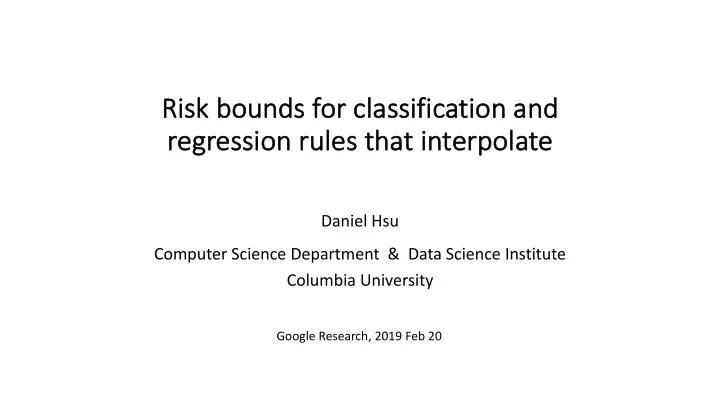
Risk bounds for cl classification and re regre ression rules that interpolate Daniel Hsu Computer Science Department & Data Science Institute Columbia University Google Research, 2019 Feb 20

Spoilers Springer Series in Statistics "A model with zero training error is Trevor Hastie overfit to the training data and will Robert Tibshirani Jerome Friedman typically generalize poorly." The Elements of Statistical Learning – Hastie, Tibshirani, & Friedman, Data Mining,Inference,and Prediction The Elements of Statistical Learning Second Edition We'll give empirical and theoretical evidence against this conventional wisdom, at least in "modern" settings of machine learning. 2

Outline 1. Statistical learning setup 2. Empirical observations against the conventional wisdom 3. Risk bounds for rules that interpolate • Simplicial interpolation • Weighted interpolated nearest neighbor (if time permits) 3

Supervised learning Training data (labeled examples) (IID from 9 ) … ! " , $ " , … , (! ' , $ ' ) from )×+ /k/ /a/ 2 ← 2 − 5∇ 7 Learning algorithm ℛ(2) Risk : ℛ - ≔ ; ℓ - ! = , $ = where !′, $′ ∼ 9 Prediction function Predicted label Test point , , !′ ∈ ) -: ) → + - !′ ∈ + /t/ 4

Modern machine learning algorithms • Choose (parameterized) function class ℱ ⊂ # $ • E.g., linear functions, polynomials, neural networks with certain architecture • Use optimization algorithm to (attempt to) minimize empirical risk / ℛ ' ≔ 1 % * + ℓ ' 1 , , 3 , ,-. (a.k.a. training error ). • But how "big" or "complex" should this function class be? (Degree of polynomial, size of neural network architecture, …) 5

Overfitting True risk Empirical risk Model complexity 6

Generalization theory • Generalization theory explains how overfitting can be avoided • Most basic form: Complexity(ℱ) %∈ℱ ℛ(*) − - ! max ℛ(*) ≲ 7 • Complexity of 8 can be measured in many ways: • Combinatorial parameter (e.g., Vapnik-Chervonenkis dimension) • Log-covering number in 9 : ; metric • Rademacher complexity (supremum of Rademacher process) • Functional / parameter norms (e.g., Reproducing Kernel Hilbert Space norm) • … 7

"Classical" risk decomposition • Let ! ∗ ∈ arg min *:,→. ℛ(!) be measurable function of smallest risk • Let 2 ∗ ∈ arg min 3∈ℱ ℛ(2) be function in ℱ of smallest risk • Then: 2 = ℛ ! ∗ + ℛ 2 ∗ − ℛ ! ∗ ℛ 5 Approximation ℛ 2 ∗ − ℛ 2 ∗ 9 + Sampling ℛ 5 9 2 − 9 ℛ 2 ∗ + Optimization + ℛ 5 ℛ 5 2 − 9 2 Generalization • Smaller ℱ : larger Approximation term, smaller Generalization term • Larger ℱ : smaller Approximation term, larger Generalization term 8

Balancing the two terms… "Sweet spot" that balances approximation and generalization True risk Empirical risk Model complexity 9

The plot thickens… Empirical observations raise new questions 10

Some observations from the field (Zhang, Bengio, Hardt, Recht, & Vinyals, 2017) Deep neural networks : • Can fit any training data. • Can generalize even when training data has substantial amount of label noise. 11

More observations from the field (Belkin, Ma, & Mandal, 2018) MNIST Kernel machines : • Can fit any training data, given enough time and rich enough feature space. • Can generalize even when training data has substantial amount of label noise. 12

Overfitting or perfect fitting? • Training produces a function ! " that perfectly fits noisy training data. • ! " is likely a very complex function! • Yet, test error of ! " is non-trivial: e.g., noise rate + 5%. Existing generalization bounds are uninformative for function classes that can interpolate noisy data. ! " chosen from class rich enough to express all possible • ways to label Ω(%) training examples. Bound must exploit specific properties of how ! " is chosen. • 13

Existing theory about local interpolation Nearest neighbor (Cover & Hart, 1967) Hilbert kernel (Devroye, Györfi, & Krzyżak, 1998) • Predict with label of nearest • Special kind of smoothing kernel training example regression (like Shepard's method) • Interpolates training data • Interpolates training data • Risk → 2 ⋅ ℛ(& ∗ ) (sort of) • Consistent, but no convergence rates 1 ) * − * , = * − * , / 14

Our goals • Counter the "conventional wisdom" re: interpolation Show interpolation methods can be consistent (or almost consistent) for classification & regression problems • Identify some useful properties of certain local prediction methods • Suggest connections to practical methods 15

New theoretical results Theoretical analyses of two new interpolation schemes 1. Simplicial interpolation • Natural linear interpolation based on multivariate triangulation • Asymptotic advantages compared to nearest neighbor rule 2. Weighted & interpolated nearest neighbor (wiNN) method • Consistency + non-asymptotic convergence rates Joint work with Misha Belkin (Ohio State Univ.) & Partha Mitra (Cold Spring Harbor Lab.) 16

Simplicial interpolation 17

Basic idea • Construct estimate ̂ " of the regression function # ' = # " # = % & ' • Regression function " is minimizer of risk for squared loss & − & , ℓ ) &, & = ) • For binary classification - = {0,1} : • " # = Pr(& ' = 1 ∣ # ' = #) • Optimal classifier : 7 ∗ # = 9 : ; < = > • We'll construct plug-in classifier ? @ # = 9 A > based on ̂ " : ; < = 18

Consistency and convergence rates Questions of interest : • What is the (expected) risk of ! " as # → ∞ ? Is it near optimal ( ℛ(( ∗ ) )? • What what rate (as function of # ) does + ℛ ! approach ℛ(( ∗ ) ? " 19

Interpolation via multivariate triangulation • IID training examples ! " , $ " , … , ! & , $ & ∈ ℝ ) ×[0,1] • Partition / ≔ conv ! " , … , ! & into simplices with ! 5 as vertices via Delaunay. • Define ̂ 7(!) on each simplex by affine interpolation of vertices' labels. • Result is piecewise linear on / . (Punt on what happens outside of / .) • For classification ( $ ∈ {0,1} ), let < = be plug-in classifier based on ̂ 7 . 20

̂ What happens on a single simplex • Simplex on ! " , … , ! '(" with corresponding labels ) " , … , ) '(" • Test point ! in simplex, with barycentric coordinates (+ " , … , + '(" ) . • Linear interpolation at ! (i.e., least squares fit, evaluated at ! ): '(" ! " . ! = 0 + 1 ) 1 ! 12" ! $ Key idea : aggregates information from all vertices to make prediction. ! # (C.f. nearest neighbor rule.) 21

Comparison to nearest neighbor rule • Suppose ! " = Pr(' = 1 ∣ ") < 1/2 for all points in a simplex • Optimal prediction of . ∗ is 0 for all points in simplex. • Suppose ' 0 = ⋯ = ' 2 = 0 , but ' 240 = 1 (due to "label noise") x 1 x 1 5 6 " = 1 here 0 0 Effect is exponentially more pronounced in high dimensions! 0 1 0 1 x 2 x 3 x 2 x 3 Nearest neighbor rule Simplicial interpolation 22

Asymptotic risk (binary classification) Theorem : Assume distribution of !′ is uniform on some convex set, and # is bounded away from 1/2 . Then simplicial interpolation's plug-in classifier ' ( satisfies 0 ℛ( ' ≤ 1 + 6 78 9 ⋅ ℛ ; ∗ limsup () / • Near-consistency in high-dimension 0 ℛ( ' ≈ 2 ⋅ ℛ ; ∗ • C.f. nearest neighbor classifier : limsup () / • "Blessing" of dimensionality (with caveat about convergence rate). • Also have analysis for regression + classification w/o condition on # 23

Weighted & interpolated NN 24

̂ Weighted & interpolated NN (wiNN) scheme • For given test point ! , let ! (#) , … , ! ' be ( nearest neighbors in training data, and let ) (#) , … , ) ' be corresponding labels. Define ' ∑ /0# 1(!, ! / ) ) / ! (#) , ! = ' ∑ /0# 1(!, ! / ) where ! ! (*) 34 , 1 !, ! / = ! − ! / 5 > 0 ! (') Interpolation : ̂ , ! → ) / as ! → ! / 25

̂ ̂ Comparison to Hilbert kernel estimate Weighted & interpolated NN Hilbert kernel (Devroye, Györfi, & Krzyżak, 1998) 9 ∑ &'( *(#, # & ) . & ) ∑ &'( *(#, # & ) . & " # = " # = 9 ∑ &'( *(#, # & ) ) ∑ &'( *(#, # & ) 12 *(#, # & ) = ‖# − # & ‖ 12 * #, # & = # − # & Our analysis needs 0 < 5 < 6/2 MUST have 5 = 6 for consistency Localization makes it possible to prove non-asymptotic rate. 26

̂ Convergence rates (regression) Theorem : Assume distribution of !′ is uniform on some compact set satisfying regularity condition, and # is $ -Holder smooth. For appropriate setting of % , wiNN estimate ̂ # satisfies ≤ ℛ # + + , -.//(./23) ' ℛ # • Consistency + optimal rates of convergence for interpolating method. • Also get consistency and rates for classification. 27