CS4495/6495 Introduction to Computer Vision 2A-L1 Images as - PowerPoint PPT Presentation
CS4495/6495 Introduction to Computer Vision 2A-L1 Images as functions Images as functions Images as functions Images as functions Images as functions Quiz An image can be thought of as: a) A 2-dimensional array of numbers ranging from some
CS4495/6495 Introduction to Computer Vision 2A-L1 Images as functions
Images as functions
Images as functions
Images as functions
Images as functions
Quiz An image can be thought of as: a) A 2-dimensional array of numbers ranging from some minimum to some maximum b) A function I of x and y: 𝐽(𝑦, 𝑧) Something generated by a camera. c) d) All of the above.
Images as functions We think of an image as a function , 𝑔 or 𝐽 , from 𝑆 2 to 𝑆 : 𝑔(𝑦, 𝑧) gives the intensity or value at position (𝑦, 𝑧)
Images as functions We think of an image as a function , 𝑔 or 𝐽 , from 𝑆 2 to 𝑆 : 𝑔(𝑦, 𝑧) gives the intensity or value at position 𝑦, 𝑧 Practically define the image over a rectangle, with a finite range: 𝑔: [𝑏, 𝑐] 𝑦 [𝑑, 𝑒] [𝑛𝑗𝑜, 𝑛𝑏𝑦]
Color images as functions A color image is just three functions “stacked” together. We can write this as a “vector - valued” function: r x y ( , ) f ( , x y ) g x y ( , ) b x y ( , ) Source: S. Seitz
The real Phyllis
Digital images In computer vision we typically operate on digital (discrete) images: Sample the 2D space on a regular grid Quantize each sample (round to “nearest integer”) Adapted from S. Seitz
Digital images Image thus represented as a matrix of integer values. Adapted from S. Seitz
j i 2D 1D Adapted from S. Seitz
Matlab – images are matrices
Matlab – images are matrices >> im = imread('peppers.png'); % semicolon or many numbers >> imgreen = im(:,:,2);
Matlab – images are matrices >> im = imread('peppers.png'); % semicolon or many numbers >> imgreen = im(:,:,2); >> imshow(imgreen) >> line([1 512], [256 256],'color','r') >> plot(imgreen(256,:)); 100 200 300 400 500 100 200 300 400 500
Noise in images • Noise is just another function that is combined with the original function to get a new – guess what – function ¢ I ( x , y ) = I ( x , y ) + h ( x , y )
Common Types of Noise Salt and pepper noise : random occurrences of black and white pixels
Common Types of Noise Impulse noise: random occurrences of white pixels
Common Types of Noise Gaussian noise : variations in intensity drawn from a Gaussian normal distribution
Gaussian noise >> noise = randn(size(im)).*sigma; >> output = im + noise; Fig: M. Hebert
Quiz: Effect of σ on Gaussian noise Noise images : Images noise = randn(size(im)).*sigma showing noise values generated with different sigma sigma = sigma = 𝜏 = 2, 8, 32, 64 Guess sigma for each noise image sigma = sigma =
Quiz: Effect of σ on Gaussian noise Noise images : Images noise = randn(size(im)).*sigma showing noise values generated with different sigma sigma = 32 sigma = 8 𝜏 = 2, 8, 32, 64 Guess sigma for each noise image sigma = 64 sigma = 2
Values of σ to use • A 𝜏 of 1.0 would be tiny if the range is [0 255] but huge if pixels went from [0.0 1.0]. • Matlab can do either and you need to be very careful - if in doubt convert to doubles.
Displaying images in Matlab Look at the Matlab function imshow() imshow(im,[LOW HIGH]) will display the image im with value LOW as black and HIGH as white.
Displaying images in Matlab Look at the Matlab function imshow() imshow(im,[]) will display the image im with the based on the range of pixel values in im .
Quiz When adding noise to images as arithmetic operators we have to worry about: The speed of the addition operation a) The magnitude of noise compared to the range of the b) image Whether we add the noise to the image or the image to c) the noise (the order of operation) None of the above d)
Recommend
More recommend
Explore More Topics
Stay informed with curated content and fresh updates.
