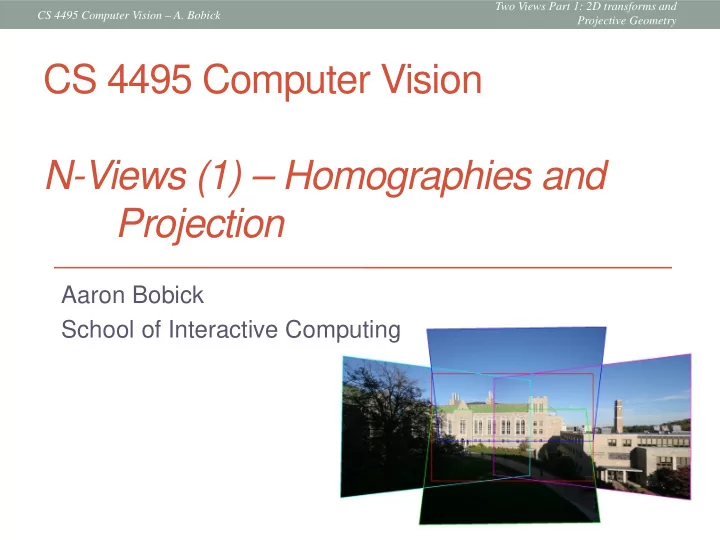

Two Views Part 1: 2D transforms and CS 4495 Computer Vision – A. Bobick Projective Geometry CS 4495 Computer Vision N-Views (1) – Homographies and Projection Aaron Bobick School of Interactive Computing
Two Views Part 1: 2D transforms and CS 4495 Computer Vision – A. Bobick Projective Geometry Administrivia • PS 2: • Get SDD and Normalized Correlation working for a given windows size – say 5x5. Then try on a few window sizes. • If too slow, resize the images (imresize) and get your code working. Then try on full images (which are reduced already!). • Results not perfect on even test images? Should they be? • Yes you can use normxcorr2 (it did say this!) • Some loops are OK. For SSD you might have 3 nested loops (row, col, disp) but shouldn’t be looping over pixels. • Now: Multiple-views • FP 7.1, 8 (all) • Today: First half of 2-Views …
Two Views Part 1: 2D transforms and CS 4495 Computer Vision – A. Bobick Projective Geometry Two views…and two lectures • Projective transforms from image to image • Some more projective geometry • Points and lines and planes • Two arbitrary views of the same scene • Calibrated – “Essential Matrix” • Two uncalibrated cameras “Fundamental Matrix” • Gives epipolar lines
Two Views Part 1: 2D transforms and CS 4495 Computer Vision – A. Bobick Projective Geometry 2D Transformations
Two Views Part 1: 2D transforms and CS 4495 Computer Vision – A. Bobick Projective Geometry 2D Transformations Example: translation tx = + ty
Two Views Part 1: 2D transforms and CS 4495 Computer Vision – A. Bobick Projective Geometry 2D Transformations Example: translation tx 1 0 tx ty . = + = ty 0 1 1
Two Views Part 1: 2D transforms and CS 4495 Computer Vision – A. Bobick Projective Geometry 2D Transformations Homogenous vector Example: translation tx 1 0 tx 1 0 tx ty . = + = . ty = 0 1 0 1 ty 1 0 0 1 [ BTW: Now we can chain transformations ]
Two Views Part 1: 2D transforms and CS 4495 Computer Vision – A. Bobick Projective Geometry Projective Transformations • Projective transformations: for 2D images it’s a 3x3 matrix applied to homogenous coordinates x ' a b c x = ' y d e f y ' w g h i w
Two Views Part 1: 2D transforms and CS 4495 Computer Vision – A. Bobick Projective Geometry Special Projective Transformations • Translation x ' 1 0 t x x = ' 0 1 y t y y 1 0 0 1 1 • Preserves: • Lengths/Areas R • Angles R • Orientation • Lines
Two Views Part 1: 2D transforms and CS 4495 Computer Vision – A. Bobick Projective Geometry Special Projective Transformations • Euclidean (Rigid body) θ − θ x ' cos( ) sin( ) t x x = θ θ ' sin( ) cos( ) y t y y 1 0 0 1 1 • Preserves: • Lengths/Areas R • Angles • Lines
Two Views Part 1: 2D transforms and CS 4495 Computer Vision – A. Bobick Projective Geometry Special Projective Transformations • Similarity (trans, rot, scale) transform θ − θ x ' a cos( ) a sin( ) t x x = θ θ ' sin( ) cos( ) y a a t y y 1 0 0 1 1 • Preserves: • Ratios of Areas R • Angles • Lines
Two Views Part 1: 2D transforms and CS 4495 Computer Vision – A. Bobick Projective Geometry Special Projective Transformations • Affine transform x ' a b c x = ' y d e f y 1 0 0 1 1 • Preserves: • Parallel lines R • Ratio of Areas • Lines
Two Views Part 1: 2D transforms and CS 4495 Computer Vision – A. Bobick Projective Geometry Projective Transformations • Remember, these are homogeneous coordinates x ' sx ' a b c x = y ' sy ' d e f y 1 s 0 0 s 1
Two Views Part 1: 2D transforms and CS 4495 Computer Vision – A. Bobick Projective Geometry Projective Transformations • General projective transform (or Homography) x ' x ' a b c x = ' ' y y d e f y 1 w ' g h i w • Preserves: • Lines R • Also cross ratios (maybe later)
Two Views Part 1: 2D transforms and CS 4495 Computer Vision – A. Bobick Projective Geometry The projective plane • What is the geometric intuition of using homogenous coordinates ? • a point in the image is a ray in projective space -y (sx,sy,s) (x,y,1) (0,0,0) x -z image plane • Each point (x,y) on the plane (at z=1) is represented by a ray (sx,sy,s) – all points on the ray are equivalent: (x, y, 1) ≅ (sx, sy, s)
Two Views Part 1: 2D transforms and CS 4495 Computer Vision – A. Bobick Projective Geometry Image reprojection The irrelevant world! • Basic question • How to relate two images from the same camera center? • how to map a pixel from projective plane PP1 to PP2 PP2 Answer • Cast a ray through each pixel in PP1 • Draw the pixel where that ray intersects PP2 PP1 Observation: Rather than thinking of this as a 3D reprojection, think of it as a 2D image warp from one image to another. Source: Alyosha Efros
Two Views Part 1: 2D transforms and CS 4495 Computer Vision – A. Bobick Projective Geometry Application: Simple mosaics Image from http://graphics.cs.cmu.edu/courses/15-463/2010_fall/
Two Views Part 1: 2D transforms and CS 4495 Computer Vision – A. Bobick Projective Geometry How to stitch together a panorama (a.k.a. mosaic)? • Basic Procedure • Take a sequence of images from the same position • Rotate the camera about its optical center • Compute transformation between second image and first • Transform the second image to overlap with the first • Blend the two together to create a mosaic • (If there are more images, repeat) • …but wait, why should this work at all? • What about the 3D geometry of the scene? • Why aren’t we using it? Source: Steve Seitz
Two Views Part 1: 2D transforms and CS 4495 Computer Vision – A. Bobick Projective Geometry Image reprojection Warning: This model only holds for angular views up to 180 ° . Beyond that need to use sequence that “bends the rays” or map onto a different surface, say, a cylinder. mosaic PP • The mosaic has a natural interpretation in 3D • The images are reprojected onto a common plane • The mosaic is formed on this plane
Two Views Part 1: 2D transforms and CS 4495 Computer Vision – A. Bobick Projective Geometry Mosaics . . . Obtain a wider angle view by combining multiple images all of which are taken from the same camera center .
Two Views Part 1: 2D transforms and CS 4495 Computer Vision – A. Bobick Projective Geometry Image reprojection: Homography • A projective transform is a mapping between any two PPs with the same center of projection • rectangle should map to arbitrary quadrilateral • parallel lines aren’t • but must preserve straight lines PP2 • called Homography wx' * * * x = PP1 wy' * * * y * * * w 1 p’ H p Source: Alyosha Efros
Two Views Part 1: 2D transforms and CS 4495 Computer Vision – A. Bobick Projective Geometry Homography ( ) ( ) ′ ′ 1 , y x x 1 , y 1 1 ( ) ′ ′ ( ) x 2 , y x 2 , y 2 2 … … ( ) ( ) ′ , ′ x n y x , n y n n To compute the homography given pairs of corresponding points in the images, we need to set up an equation where the parameters of H are the unknowns…
Two Views Part 1: 2D transforms and CS 4495 Computer Vision – A. Bobick Projective Geometry Solving for homographies p’ = Hp wx' a b c x = wy' d e f y w g h i 1 • Can set scale factor i=1. So, there are 8 unknowns. • Set up a system of linear equations Ah = b • where vector of unknowns h = [a,b,c,d,e,f,g,h]T • Need at least 4 points for 8 eqs, but the more the better… • Solve for h. If overconstrained, solve using least-squares: 2 min Ah b - • Look familiar? (If don’t set i to 1 can use SVD) • >> help mldivide
Recommend
More recommend