Corners and Interest Points Various slides from previous courses by: - PowerPoint PPT Presentation
CS4501: Introduction to Computer Vision Corners and Interest Points Various slides from previous courses by: D.A. Forsyth (Berkeley / UIUC), I. Kokkinos (Ecole Centrale / UCL). S. Lazebnik (UNC / UIUC), S. Seitz (MSR / Facebook), J. Hays (Brown /
CS4501: Introduction to Computer Vision Corners and Interest Points Various slides from previous courses by: D.A. Forsyth (Berkeley / UIUC), I. Kokkinos (Ecole Centrale / UCL). S. Lazebnik (UNC / UIUC), S. Seitz (MSR / Facebook), J. Hays (Brown / Georgia Tech), A. Berg (Stony Brook / UNC), D. Samaras (Stony Brook) . J. M. Frahm (UNC), V. Ordonez (UVA).
Last Class • Frequency Domain • Filtering in Frequency • Edge Detection - Canny
Today’s Class • Corner Detection - Harris • Interest Points • Local Feature Descriptors
Edge Detection
Edge Detection ! ", $ = &1, ((", $) ≥ , • Sobel + Thresholding 0, ( ", $ < ,
Digression • Thresholding is often the most under-rated but effective Computer Vision technique. Sometimes this is all you need! Example: intensity-based detection. Warning when door is opened or closed. fg_pix = find(im < 65); Looking for dark pixels Example by Kristen Grauman, UT-Austin
Canny Edge Detector • Obtains thin edges (1px wide) • Tries to preserve edge connectivity. Source: Juan C. Niebles and Ranjay Krishna.
Canny edge detector 1. Filter image with x, y derivatives of Gaussian 2. Find magnitude and orientation of gradient 3. Non-maximum suppression: Thin multi-pixel wide � ridges � down to single pixel width • 4. Thresholding and linking (hysteresis): Define two thresholds: low and high • Use the high threshold to start edge curves and the low threshold to • continue them Source: Juan C. Niebles and Ranjay Krishna.
Canny Edge Detector • Classic algorithm in Computer Vision / Image Analysis • Commonly implemented in most libraries • e.g. in Python you can find it in the skimage package. OpenCV also has an implementation with python bindings. Canny, J., A Computational Approach To Edge Detection , IEEE Trans. Pattern Analysis and Machine Intelligence, 8(6):679–698, 1986.
Corners (and Interest Points) • How to find corners? • What is a corner?
Corners: Why “Interest” Points? If we can find them, then maybe we can “match” images belonging to the same object! Then maybe we can also “triangulate” the 3D coordinates of the image. Example from Silvio Savarese
Corner Detection: Basic Idea •We should easily recognize the point by looking through a small window •Shifting a window in any direction should give a large change in intensity “flat” region: “edge”: “corner”: no change in no change significant all directions along the edge change in all direction directions Source: A. Efros
Harris Corner Detection • Compute the following matrix of squared gradients for every pixel. $ % are gradients $ ' and & $ % $ % $ ' ! = # computed using Sobel or & $ ' $ % $ ' some other approximation. ()*+, ! = / 0 ! = / 0 ! = 0 0 ! = 0 0 0 0 0 . 0 0 0 .
Harris Corner Detection ! = % 0 ! = % 0 ! = 0 0 ! = 0 0 0 0 0 $ 0 0 0 $ • If both a, and b are large then this is a corner, otherwise it is not. Set a threshold and this should detect corners. Problem: Doesn’t work for these corners:
Harris Corner Detection & $ % $ % $ ' = ( ) ! = # ) * & $ ' $ % $ ' +,-./ 23 4 3 0 Under a rotation M can be diagonalized ! = 0 1 4 & 0 1 0 4 3 and 4 & are the eigenvalues of M det ! − 4$ = 0 From your linear algebra class finding them requires solving
However no need to solve det(M-lambda I)=0 = l l det M 1 2 = l + l trace M 1 2
Corner response function = - a = l l - a l + l 2 2 R det( M ) trace ( M ) ( ) 1 2 1 2 α : constant (0.04 to 0.06) “Edge” R < 0 “Corner” R > 0 |R| small “Edge” “Flat” R < 0 region
Harris Detector Summary [ Harris88 ] • Second moment matrix é ù s s 2 I ( ) I I ( ) µ s s = s * x D x y D 1. Image I x I y ( , ) g ( ) ê ú I D I s 2 s I I ( ) I ( ) ê ú derivatives ë û x y D y D (optionally, blur first) I y I x I y I x 2. Square of 2 2 derivatives = l l det M 1 2 = l + l trace M g(I x I y ) 1 2 g(I x2 ) g(I y2 ) 3. Gaussian filter g( s I ) 4. Cornerness function – both eigenvalues are strong = µ s s - a µ s s = 2 har det[ ( , )] [trace( ( , )) ] I D I D - - a + 2 2 2 2 2 2 g ( I ) g ( I ) [ g ( I I )] [ g ( I ) g ( I )] x y x y x y 5. Non-maxima suppression 18 har
Alternative Corner response function “edge”: “corner”: “flat” region l 1 >> l 2 l 1 and l 2 are large, l 1 and l 2 are small; l 1 ~ l 2 ; l 2 >> l 1 = l l det M Szeliski 1 2 = l + l trace M Harmonic mean 1 2
Harris Detector: Steps
Harris Detector: Steps Compute corner response R
Harris Detector: Steps Find points with large corner response: R> threshold
Harris Detector: Steps Take only the points of local maxima of R
Harris Detector: Steps
Invariance and covariance • We want corner locations to be invariant to photometric transformations and covariant to geometric transformations • Invariance: image is transformed and corner locations do not change • Covariance: if we have two transformed versions of the same image, features should be detected in corresponding locations Slide by James Hays
Keypoint detection with scale selection • We want to extract keypoints with characteristic scale that is covariant with the image transformation Slide by Svetlana Lazebnik
Basic idea Convolve the image with a “blob filter” at multiple • scales and look for extrema of filter response in the resulting scale space T. Lindeberg. Feature detection with automatic scale selection. IJCV 30(2), pp 77-116, 1998. Slide by Svetlana Lazebnik
Blob detection minima = * maxima • Find maxima and minima of blob filter response in space and scale Source: N. Snavely
Blob filter • Laplacian of Gaussian: Circularly symmetric operator for blob detection in 2D ¶ ¶ 2 2 g g Ñ = + 2 g ¶ ¶ 2 2 x y
Recall: Edge detection Edge f d Derivative g of Gaussian dx d Edge = maximum f * g of derivative dx Source: S. Seitz
Edge detection, Take 2 Edge f Second derivative 2 d of Gaussian g 2 (Laplacian) dx 2 d Edge = zero crossing * f g of second derivative 2 dx Source: S. Seitz
Scale-space blob detector 1. Convolve image with scale-normalized Laplacian at several scales
Scale-space blob detector: Example Slide by Svetlana Lazebnik
Scale-space blob detector: Example Slide by Svetlana Lazebnik
Scale-space blob detector 1. Convolve image with scale-normalized Laplacian at several scales 2. Find maxima of squared Laplacian response in scale-space Slide by Svetlana Lazebnik
Scale-space blob detector: Example Slide by Svetlana Lazebnik
Eliminating edge responses Laplacian has strong response along edge • Slide by Svetlana Lazebnik
Efficient implementation Approximating the Laplacian with a difference of Gaussians: • ( ) = s 2 s + s L G ( , , ) x y G ( , , ) x y xx yy (Laplacian) = s - s DoG G x y k ( , , ) G x y ( , , ) (Difference of Gaussians) Slide by Svetlana Lazebnik
Efficient implementation David G. Lowe. "Distinctive image features from scale-invariant keypoints.” IJCV 60 (2), pp. 91-110, 2004.
SIFT keypoint detection D. Lowe, Distinctive image features from scale-invariant keypoints, IJCV 60 (2), pp. 91-110, 2004.
Questions? 41
Recommend
More recommend
Explore More Topics
Stay informed with curated content and fresh updates.
