Cooperative Data Analysis in Supply Chains Using Selective - PowerPoint PPT Presentation
Cooperative Data Analysis in Supply Chains Using Selective Information Disclosure JRG LSSIG 1 AND MICHAEL HAHSLER 2 1 University of Applied Sciences Zittau/Grlitz, Germany 2 Southern Methodist University, Dallas, Texas INFORMS Computing
Cooperative Data Analysis in Supply Chains Using Selective Information Disclosure JÖRG LÄSSIG 1 AND MICHAEL HAHSLER 2 1 University of Applied Sciences Zittau/Görlitz, Germany 2 Southern Methodist University, Dallas, Texas INFORMS Computing Society Conference Richmond, VA January 2015
Photo: www.ifixit.com Global supply chain with many suppliers Products become more complex Finding defects requires access to data for analysis Exact production processes are complicated and may be confidential Effective strategies for cooperative data analysis using selective data disclosure.
Background Privacy preserving data mining (Aggarwal & Yu 2008, Lindell & Pinkas 2000) – Protect private information (age, income, etc.) – Aim: Statistical data analysis on the aggregate Companies participating in a supply chain – Incentive to share (mostly logistics) information (Huang, Lau & Mak 2003, Subramani 2004) – Competition can hinder information sharing (Li 2002, Frohlich 2002) – Information protection goals are different than for companies – Root cause analysis (RCA) needs not just logistics information • Details about a proprietary production process • Change of a third party supplier • Large volume of very detailed data → Trade -off: Minimize necessary information exchange
Supply Chain • A directed acyclic graph G = (V, E) • Participants V • Material and information flows E Class information known to s Vertically partitioned data set 𝓤
Protocols for Optimized Information Disclosure 𝑈 𝑈 Trivial case 𝑤1 𝑤3 – Single party or full disclosure Direct case – Scenario 1: Known supplier 𝑑 𝑑 – Scenario 2: Supplier not known – Scenario 3: Interaction between suppliers Remote case 𝑑 – Propagate the class information – Recursive application of Direct case 𝑑 𝑑 Information flow
Direct Case Scenario 1 : Known supplier – Supplier v receives class information for analysis. – Addresses problems and/or reports results to s. Scenario 2 : Supplier not known – All direct suppliers receive class information for analysis. – One supplier finds a strong association addresses problem and notifies s. Scenario 3 : Interaction between suppliers – Like scenario 2, but several supplier find (weaker) associations. – Further analysis can be coordinated by s.
Analyzing Dependencies Many methods are available for root cause analysis Statistical analysis – Contingency tables and Chi-square test – (rank) correlation Data mining (Tan, Steinbach & Kumar, 2006) – Classification model • Decision trees, logistic regression, SVM, etc. • Variable importance – Association analysis • Association rule mining
Association Rules X → class Create transactions – 𝑈 𝑤1 ⋈ 𝑑 𝑢 1,1 = 𝑛𝑛 𝑢 1,1 = 𝑛 2 𝑢 1,1 = 𝑛 3 𝑢 1,2 = 𝑡𝑛 𝑢 1, 𝑛 ( 𝑤 1 ) = 𝑛 1 𝒅 … 𝑢 1 1 0 0 0 … 0 1 𝑢 2 0 0 1 0 … 0 0 … … … … … … … … 𝑢 | 𝐿 | 1 0 0 0 … 1 1
Association Rules X → class 𝑢 1,1 = 𝑛𝑛 𝑢 1,1 = 𝑛 2 𝑢 1,1 = 𝑛 3 𝑢 1,2 = 𝑡𝑛 𝑢 1, 𝑛 ( 𝑤 1 ) = 𝑛 1 𝒅 … 𝑢 1 1 0 0 0 … 0 1 𝑢 2 0 0 1 0 … 0 0 … … … … … … … … 𝑢 | 𝐿 | 1 0 0 0 … 1 1 Support/confidence framework (Agrawal, Imielinski & Swami, 1993) Set of items: I = { 𝑢 1 , 1 = 𝑛𝑛 , 𝑢 1 , 2 = 𝑛 2 , … , 𝑢 1 , 𝑛 ( 𝑤 1 ) = 𝑛𝑛 } Left hand side of rule: 𝑌 ⊆ I Rule: 𝑌 → 𝑑 𝑙∈ 1 , 2 ,…, 𝐿 ; 𝑌∪𝑑 ⊆𝑢 𝑙 Support: sup 𝑌 → 𝑑 = > 𝜏 | 𝐿 | sup 𝑌 ∪ 𝑑 Confidence: 𝑑𝑑𝑑𝑑 𝑌 → 𝑑 = > 𝛿 sup ( 𝑌 )
Association Rules X → class � 𝒀 𝒀 One-sided Fisher's exact test to measure the 𝑑 strength of rules (Hahsler & Hornik, 2007). 100 3 Accept associations with a p -value < α � 𝑑 3000 400000 Correction for multiple comparisons (Miller, 1981) – Bonferroni Correction: 𝛽 = 𝛽 ∗ α … test sig. level α * … family wise sig. 𝑛 m … # of tests Number of shared tuples n=| Γ | represent a sample. – Upper limit on sample size based on Chernoff bounds (Zaki et al., 1997): ε … error rate 1-c … confidence level τ … support
Simulation Study Chernoff bounds give 240,000 at 1% Scenario 1: Known supplier support and – Simple case of Scenario 2 confidence and Scenario 2: Supplier not known accuracy level of 95% Scenario 3: Interaction between 2 suppliers – Like Scenario 2, but several supplier find (weak) associations. – Further analysis can be coordinated by s.
Amount of Shared Information Avg: 744 unique features values Fixed at | Γ | x |V|
Scenario 2: Supplier not known Finding less frequent errors takes more data. Selective disclosure is as effective as complete disclosure. Selective disclosure incorrectly reports more features due to undercorrection.
Scenario 3: Interaction between 2 suppliers Same as for Scenario 2: Finding less frequent errors takes more data. Selective disclosure is as effective as complete disclosure. Selective disclosure incorrectly reports more features due to undercorrection.
Deployment Easy to use plug-in for • https://rapidminer.com/ RapidMiner. Central coordination web • service to model supply chain. Secure communication • directly between participants. Participants have full • control over what information is shared. Direct secure communication
Conclusion Many modern products are complicated and error-prone. Data to perform root cause analysis is often not shared in supply chains. Selective information disclosure: – Addresses need to performs distributed data analysis – Minimizes the amount of data to be exposed – Can be automated such that participants do not need to have in-depth data analysis capabilities – Initial experiments suggest that it can be effective
Thank you for your attention! Michael Hahsler mhahsler@lyle.smu.edu
Recommend
More recommend
Explore More Topics
Stay informed with curated content and fresh updates.
