Attempting to measure the power spectrum of radio anisotropies by - PowerPoint PPT Presentation

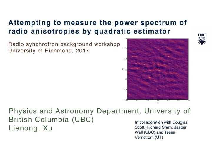
Attempting to measure the power spectrum of radio anisotropies by quadratic estimator Radio synchrotron background workshop University of Richmond, 2017 Physics and Astronomy Department, University of British Columbia (UBC) In collaboration with Douglas Lienong, Xu Scott, Richard Shaw, Jasper Wall (UBC) and Tessa Vernstrom (UT) 1

Radio power spectrum • Scientific purpose, motivation • Method and procedure • Testing with simulated data • Preliminary result from real data • Next steps 2

Scientific Purposes and Motivations • Complementary to radio synchrotron isotropy (monopole) • Detect and trace the anisotropic extragalactic synchrotron emissions (in GHz from 0.1arcmin to 0.1deg) • The Cosmic Web in synchrotron • Understand how radio emission fits into structure formation • Use tools from CMB and CIB anisotropy studies • Use likelihood approach with quadratic estimators • The well-known radio/FIR correlation means we know roughly what to expect • Develop a general-purpose tool for estimating power spectra from radio interferometric data 3

Scientific Purposes and Motivations Regular approach of measuring the power spectrum include: • Observe and measure visibility data • Produce radio images • Compute correlation function • Fourier power spectrum 4

Scientific Purposes and Motivations Alternatively, radio visibility data is ‘already’ measured in Fourier domain, i.e. uv-space. The (angular) power spectrum is also defined in Fourier space. Therefore it worth trying to directly extract the radio power spectrum from the measured visibility data, at least without having to construct radio images. Consequently it reduce the error propagation with less steps and increase the performance of interferometric data (will delete it in my own word) 5

Method and Procedures • Grid the uv-visibility plane • Apply the quadratic estimator • Construct dirty map (not necessary) • Noise estimation • Attempt with single pointing measurement 6

Model the sky angular power spectrum Assume the sky is Gaussian random field with power spectrum D E T ( u ) ˜ ˜ = C ( u ) δ 2 ( u − u 0 ) T ⇤ ( u 0 ) • T(u) is the Fourier transform of the radio sky temperature T(x). • The relation of u and multipole number l is: l + 1 / 2 = 2 π u And the C(u) is related to by: C l C ( u ) = C 2 ⇡ u ≈ C ` (Myers, 2003) 7

Measured visibility and radio image • The antennas keep tracking at the phase centre x k • The perceived visibility is the Fourier transform of the sky temperature convolved with the primary beam Z d 2 x A ( x − x k ) e − 2 π i u i · ( x − x k ) T ( x ) , V k i = Define the (inverse) Fourier transform of the primary beam and sky temperature as follows (Flat sky approximation): Z d 2 u ˜ A ( u ) e 2 π i u · x A ( x ) = Z d 2 u ˜ T ( u ) e 2 π i u · x T ( x ) = (Myers, 2003) 8

Measured visibility and radio image Obtain the expression of visibility as an integration in uv-space: Z A ( u i − u ) e 2 π i u · x k ˜ d 2 u ˜ V k i = T ( u ) Discretize the above integration in to summation and formulate as a matrix- vector operation v = Bt + n Each component stores the sky temperature at one grid position. B is the response matrix which transforms the sky temperature into visibility data: [ B ] ( kij ) = ˜ A ( u i − u j ) e 2 π i u j · x k (Myers, 2003) 9

Gridded temperature plane T ( u ) • T(u) has same number of grids (pixels) as the radio image T(x) • is not the quantity measured directly • is the quantity related to power spectrum 10

Modelling the power spectrum Each component of visibility vector is the visibility measurement at one frequency, at a particular uv position with antenna pointing at chosen phase centre . x k v = Bt + n Recall the definition of power spectrum: D E T ( u ) ˜ ˜ = C ( u ) δ 2 ( u − u 0 ) T ⇤ ( u 0 ) The matrix version of the power spectrum is: (Tegmark, 1997) X t t † ↵ ⌦ p a P a = a Here the power spectrum is binned into different band power. represents p a p a fluctuation amplitude of the angular mode. The sets of are the parameters going to be estimated. 11

Modelling the power spectrum X t t † ↵ ⌦ p a P a = a ( 1 i = j and u a − 1 < | u i | < u a [ P a ] ij = 0 otherwise The total visibility data covariance is: vv † ↵ ⌦ C = Assume the noise is independent and uncorrelated with the signal, the data covariance matrix is expressed as: B † + tt † ↵ nn † ↵ ⌦ ⌦ C = B a p a BP a B † + N X = X a p a C a + N = (Tegmark, 1997) C a = BP a B † 12

Quadratic Estimator p a Employ the quadratic estimator framework for by X p a = ˆ M ab (ˆ q b − b b ) b q a = 1 2 v † E a v ˆ The matrix are undetermined. They group the pairs of visibility data E a with different weight to estimate the band power. If the visibility data is Gaussian, the covariance of the power spectrum parameter is: p b ) = 1 X Cov(ˆ p a , ˆ M ac M bd Tr [ E c CE d C ] 2 cd (Tegmark, 1997) 13

Quadratic estimator, constraints Want the estimator to be unbiased: h ˆ p a i = p a Therefore: b a = 1 2 Tr [ E a N ] M ab Tr [ E b C b ] = 2 δ ab (Tegmark, 1997) 14

Quadratic estimator constraints Want the parameters are estimated with minimum variance, the optimal solution correspond to inverse variance weighting. E a = C − 1 C a C − 1 Recall the definition of the Fisher matrix (with zero mean): F ab = 1 C a C − 1 C b C − 1 ⇤ ⇥ 2 Tr With inverse variance weighted solution, the mixing matrix M is the inverse of Fisher matrix: M ab = F − 1 (Tegmark, 1997) ab 15

Quadratic estimator procedure Consequently the parameter covariance also equals to the inverse of Fisher matrix. p b ) = F − 1 Cov(ˆ p a , ˆ ab All it needs is an initial fiducial model for power spectrum and data covariance matrix to approximate the Fisher matrix and then update the Fisher matrix and band power parameter iteratively (Tegmark, 1997) 16

Dirty map (not necessary) • Image reconstruction is not critical in this approach. The idea of reconstruction is to recover the radio image from visibility data, i.e. invert the previous equation: v = Bt + n • The maximum likelihood of sky estimate turns out to be the Wiener filter solution t t † ↵ − 1 + B † N − 1 B ) − 1 ˆ B † N − 1 v ⌦ t = ( • However if the sky covariance is not known in prior, the exact solution cannot be calculated. As an approximation, keep the numerator only. t = B † N − 1 v ˆ (Seljak, 1997) • This dirty map equation only works for a consistency check. 17

Data: ATCA & SKA simulate skies • Australia Telescope Compact Array (ATCA) • ELAIS-S1 region centres at RA=1.4h / Dec = -43 deg Frequencies: from 1.08 GHz to 2.09 GHz, 64 channels • • uv-spacing: from 30m to 350m • 5 antennas in operation Integration time = 10 seconds Observation time = 10 hours Assumptions: identical aperture, Gaussian primary ATCA beam, Gaussian random field, and Gaussian error. 18

Data: ATCA & SKA simulate skies • SKA simulated sky S^3 simulation at 1.4GHz (Wilman,2008) • Use the flux density distribution from the simulated point sources • Create multifrequency data by single spectral index -0.7 • Distribute the position of the sources randomly or clustered. • Add extended / diffuse emission feature by convolving Gaussian in arcmin scale. 19

ATCA Visibility measurement Measurement of one pair of antennas, at one frequency, during the observation time. Simulation of two point sources 20

ATCA uv coverage All baselines at a single frequency 21

ATCA uv coverage All baselines at a single frequency 22

ATCA uv coverage All baselines at all frequencies in dimensionless uv baselines 23

Checks for a point source image • Simulate a point source image • Calculate the ‘measured’ visibility • Dirty map • Power spectrum 24

Checks for a point source image Dirty map: point spread function 25

Point source power spectrum l max l min l = 2 π | u | 26

Result from simulated sky A realistic simulation to practice Determine if clustering can be detected (even in principle). Can calculate power spectrum for • both point sources + extended emission • point sources only • extended emission only • Point sources can be distributed either randomly or clustered 27

Poisson random point sources only 28

Extended emission only 29

Poisson point sources + extended emission 30

Clustered point sources only 31

Extended emission only 32

Clustered point sources + extended emission 33

Noise estimation: null test • Split the data into even and odd frequency • Split the data into even and odd time measurement • Monte Carlo simulation • Stokes V Important for auto-power spectrum estimation 34

Null test: split in frequency bands 35

Null test power spectrum Difference of the power spectrum 36

Preliminary results from ATCA real visibility data • Seven sets of visibility data forming a hexagonal field of view 37

I am still checking the reliability of the results The other six 38

Next steps • Careful analysis of noise, errors • Implementation of mosaicking • Testing with more sizeble data: VLA • Expecting more suitable observation 39