Contours and Regions Pablo Arbelez UC Berkeley I. HISTORICAL - PowerPoint PPT Presentation
Contours and Regions Pablo Arbelez UC Berkeley I. HISTORICAL MOTIVATION Some Computer Vision Prehistory Hubel and Wiesel (1981 Nobel Price winners): MEASUREMENT system INPUT Selective response: Physiological evidence for the
Normalized Cuts ◮ Graph G = ( V , E , W ) ◮ Split into A , B disjoint, A ∪ B = V � � cut ( A , B ) = w ( u , v ) assoc ( A , V ) = w ( u , v ) u ∈ A , v ∈ B u ∈ A , v ∈ V cut ( A , B ) cut ( A , B ) Ncut ( A , B ) = assoc ( A , V ) + assoc ( B , V ) ◮ General case: partition using smallest eigenvectors of ( D − W ) v = λ Dv where D ii = � j W ij J. Shi and J. Malik. “Normalized Cuts and Image Segmentation”, PAMI, 2000.
Do NOT Cluster Eigenvectors! Clustering eigenvector Image values leads to artifacts on uniform regions. Eigenvectors
Eigenvectors Carry Contour Information We use the gradients of Image eigenvectors rather than their values. Eigenvectors
Eigenvectors Carry Contour Information Gradients of eigenvectors indicate salient contours in the image.
Contour Detection ◮ Multiscale Brightness, Color, Texture Gradients: � � mPb ( x , y , θ ) = α i , s G i ,σ ( s ) ( x , y , θ ) s i
Contour Detection ◮ Multiscale Brightness, Color, Texture Gradients: � � mPb ( x , y , θ ) = α i , s G i ,σ ( s ) ( x , y , θ ) s i ◮ Gradients of Eigenvectors: 1 � √ λ k sPb ( x , y , θ ) = · ∇ θ v k ( x , y ) k
Contour Detection ◮ Multiscale Brightness, Color, Texture Gradients: � � mPb ( x , y , θ ) = α i , s G i ,σ ( s ) ( x , y , θ ) s i ◮ Gradients of Eigenvectors: 1 � √ λ k sPb ( x , y , θ ) = · ∇ θ v k ( x , y ) k ◮ Global Probability of Boundary: � � gPb ( x , y , θ ) = β i , s G i ,σ ( s ) ( x , y , θ ) + γ · sPb ( x , y , θ ) s i
Contour Detection ◮ Multiscale Brightness, Color, Texture Gradients: � � mPb ( x , y , θ ) = α i , s G i ,σ ( s ) ( x , y , θ ) s i ◮ Gradients of Eigenvectors: 1 � √ λ k sPb ( x , y , θ ) = · ∇ θ v k ( x , y ) k ◮ Global Probability of Boundary: � � gPb ( x , y , θ ) = β i , s G i ,σ ( s ) ( x , y , θ ) + γ · sPb ( x , y , θ ) s i Weights learned from training data
Benefits of Globalization Thresholded Pb Thresholded gPb
Benefits of Globalization Thresholded Pb Thresholded gPb
Benefits of Globalization 1 iso−F 0.9 0.9 0.8 0.7 0.8 0.6 Precision 0.7 0.5 0.6 0.4 0.5 0.3 0.4 0.2 0.3 [F = 0.79] Human [F = 0.70] gPb 0.2 0.1 [F = 0.68] sPb [F = 0.67] mPb 0.1 [F = 0.65] Pb − Martin, Fowlkes, Malik (2004) 0 0 0.1 0.2 0.3 0.4 0.5 0.6 0.7 0.8 0.9 1 Recall
Contours to Hierarchical Regions
Contours to Hierarchical Regions pb OWT-UCM Segmentation
Watershed Transform ◮ Compute pb ( x , y ) = max θ pb ( x , y , θ )
Watershed Transform ◮ Compute pb ( x , y ) = max θ pb ( x , y , θ ) ◮ Seed locations are regional minima of pb ( x , y )
Watershed Transform ◮ Compute pb ( x , y ) = max θ pb ( x , y , θ ) ◮ Seed locations are regional minima of pb ( x , y ) ◮ Apply watershed transform
Watershed Transform ◮ Compute pb ( x , y ) = max θ pb ( x , y , θ ) ◮ Seed locations are regional minima of pb ( x , y ) ◮ Apply watershed transform ◮ Catchment basins P 0 are regions
Watershed Transform ◮ Compute pb ( x , y ) = max θ pb ( x , y , θ ) ◮ Seed locations are regional minima of pb ( x , y ) ◮ Apply watershed transform ◮ Catchment basins P 0 are regions ◮ Arcs K 0 are boundaries
Oriented Watershed Transform (OWT) pb ( x , y ) Watershed
Oriented Watershed Transform (OWT) pb ( x , y ) Watershed Subdivision
Oriented Watershed Transform (OWT) pb ( x , y , θ ) Watershed Subdivision
Oriented Watershed Transform (OWT) pb ( x , y , θ ) OWT Subdivision
Oriented Watershed Transform (OWT) pb ( x , y , θ ) OWT Watershed
Ultrametric Contour Map (UCM) ◮ Duality between closed, non-self-intersecting weighted contours and a hierarchy of regions 1 1 P. Arbel´ aez. “Boundary Extraction in Natural Images using Ultrametric Contour Maps”, POCV, 2006.
Ultrametric Contour Map (UCM) ◮ Duality between closed, non-self-intersecting weighted contours and a hierarchy of regions 1 ◮ Graph G = ( P 0 , K 0 , W ( K 0 )) given by OWT 1 P. Arbel´ aez. “Boundary Extraction in Natural Images using Ultrametric Contour Maps”, POCV, 2006.
Ultrametric Contour Map (UCM) ◮ Duality between closed, non-self-intersecting weighted contours and a hierarchy of regions 1 ◮ Graph G = ( P 0 , K 0 , W ( K 0 )) given by OWT ◮ Iteratively merge regions by removing minimum weight boundary 1 P. Arbel´ aez. “Boundary Extraction in Natural Images using Ultrametric Contour Maps”, POCV, 2006.
Ultrametric Contour Map (UCM) ◮ Duality between closed, non-self-intersecting weighted contours and a hierarchy of regions 1 ◮ Graph G = ( P 0 , K 0 , W ( K 0 )) given by OWT ◮ Iteratively merge regions by removing minimum weight boundary ◮ Produces region tree ◮ Root is entire image ◮ Leaves are P 0 ◮ Height ( R ) is boundary threshold at which R first appears ◮ Distance ( R 1 , R 2 ) = min { Height ( R ) : R 1 , R 2 ⊆ R } 1 P. Arbel´ aez. “Boundary Extraction in Natural Images using Ultrametric Contour Maps”, POCV, 2006.
Ultrametric Contour Map (UCM)
Ultrametric Contour Map (UCM)
Ultrametric Contour Map (UCM)
OWT-UCM Preserves Boundary Quality 1 iso−F 0.9 0.9 0.8 0.7 0.8 0.6 Precision 0.7 0.5 0.6 0.4 0.5 0.3 0.4 0.2 0.3 [F = 0.79] Human [F = 0.71] gPb−owt−ucm 0.2 0.1 [F = 0.70] gPb [F = 0.58] Canny−owt−ucm 0.1 [F = 0.58] Canny 0 0 0.1 0.2 0.3 0.4 0.5 0.6 0.7 0.8 0.9 1 Recall
Hierarchical Segmentation Results gPb -owt-ucm ODS OIS
Hierarchical Segmentation Results gPb -owt-ucm ODS OIS
Empirical Evaluation
Benchmarking Region Boundaries 1 iso−F 0.9 0.9 0.8 0.7 0.8 0.6 Precision 0.7 0.5 0.6 0.4 0.5 0.3 [F = 0.79] Human [F = 0.71] gPb−owt−ucm 0.4 [F = 0.67] UCM − Arbelaez (2006) [F = 0.63] Mean Shift − Comaniciu, Meer (2002) 0.2 [F = 0.62] Normalized Cuts − Cour, Benezit, Shi (2005) 0.3 [F = 0.58] Canny−owt−ucm [F = 0.58] Felzenszwalb, Huttenlocher (2004) [F = 0.58] Av. Diss. − Bertelli, Sumengen, Manjunath, Gibou (2008) 0.2 0.1 [F = 0.55] ChanVese − Bertelli, Sumengen, Manjunath, Gibou (2008) [F = 0.55] Donoser, Urschler, Hirzer, Bischof (2009) 0.1 [F = 0.53] Yang, Wright, Ma, Sastry (2007) 0 0 0.1 0.2 0.3 0.4 0.5 0.6 0.7 0.8 0.9 1 Recall
Region Quality ◮ Segmentation methods burdened with the constraint of producing closed boundaries
Region Quality ◮ Segmentation methods burdened with the constraint of producing closed boundaries ◮ BSDS boundary benchmark might favor contour detectors
Region Quality ◮ Segmentation methods burdened with the constraint of producing closed boundaries ◮ BSDS boundary benchmark might favor contour detectors ◮ Region-based performance metrics
Region Quality ◮ Segmentation methods burdened with the constraint of producing closed boundaries ◮ BSDS boundary benchmark might favor contour detectors ◮ Region-based performance metrics ◮ Variation of Information
Region Quality ◮ Segmentation methods burdened with the constraint of producing closed boundaries ◮ BSDS boundary benchmark might favor contour detectors ◮ Region-based performance metrics ◮ Variation of Information ◮ Rand Index
Region Quality ◮ Segmentation methods burdened with the constraint of producing closed boundaries ◮ BSDS boundary benchmark might favor contour detectors ◮ Region-based performance metrics ◮ Variation of Information ◮ Rand Index ◮ Segmentation Covering
Variation of Information Distance between two clusterings of data C and C ′ given by VI ( C , C ′ ) = H ( C ) + H ( C ′ ) − 2 I ( C , C ′ ) Here C and C ′ are test and ground-truth segmentations.
Probabilistic Rand Index Given a set of ground-truth segmentations { G k } , PRI ( S , { G k } ) = 1 � [ c ij p ij + (1 − c ij )(1 − p ij )] T i < j where c ij is the event that pixels i and j have the same label and p ij its probability.
Segment Covering Overlap between two regions R and R ′ : O ( R , R ′ ) = | R ∩ R ′ | | R ∪ R ′ | Covering of a segmentation S by a segmentation S ′ : C ( S ′ → S ) = 1 � R ′ ∈ S ′ O ( R , R ′ ) | R | · max N R ∈ S We report the covering of groundtruth by test.
Region Benchmarks on the BSDS Covering PRI VI ODS OIS Best ODS OIS ODS OIS Human 0 . 73 0 . 73 − 0 . 87 0 . 87 1 . 16 1 . 16 gPb - owt - ucm 0 . 59 0 . 65 0 . 75 0 . 81 0 . 85 1 . 65 1 . 47 Mean Shift 0 . 54 0 . 58 0 . 66 0 . 78 0 . 80 1 . 83 1 . 63 Felz - Hutt 0 . 51 0 . 58 0 . 68 0 . 77 0 . 82 2 . 15 1 . 79 Canny - owt - ucm 0 . 48 0 . 56 0 . 66 0 . 77 0 . 82 2 . 11 1 . 81 NCuts 0 . 44 0 . 53 0 . 66 0 . 75 0 . 79 2 . 18 1 . 84 Total Var. 0 . 57 − − 0 . 78 − 1 . 81 − T+B Encode 0 . 54 − − 0 . 78 − 1 . 86 − Av. Diss. 0 . 47 − − 0 . 76 − 2 . 62 − ChanVese 0 . 49 − − 0 . 75 − 2 . 54 −
Interactive Segmentation ◮ Relevant for graphics applications
Interactive Segmentation ◮ Relevant for graphics applications ◮ Graph cuts formalism has become popular 1 , 2 , 3 ◮ User marks foreground/background ◮ Region model learned on the fly 1 Y. Boykov and M.-P. Jolly. “Interactive Graph Cuts for Optimal Boundary & Region Segmentation of Objects in N-D Images”, ICCV, 2001 3 C. Rother, V. Kolmogorov, A. Blake. ““Grabcut”: Interactive Foreground Extraction using Iterated Graph Cuts”, SIGGRAPH, 2004 2 Y. Li, J. Sun, C.-K. Tang, and H.-Y. Shum. “Lazy Snapping”, SIGGRAPH, 2004
Interactive Segmentation ◮ Relevant for graphics applications ◮ Graph cuts formalism has become popular 1 , 2 , 3 ◮ User marks foreground/background ◮ Region model learned on the fly 1 Y. Boykov and M.-P. Jolly. “Interactive Graph Cuts for Optimal Boundary & Region Segmentation of Objects in N-D Images”, ICCV, 2001 3 C. Rother, V. Kolmogorov, A. Blake. ““Grabcut”: Interactive Foreground Extraction using Iterated Graph Cuts”, SIGGRAPH, 2004 2 Y. Li, J. Sun, C.-K. Tang, and H.-Y. Shum. “Lazy Snapping”, SIGGRAPH, 2004 ◮ Alternative: use precomputed segmentation tree 4 ◮ Distance ( R 1 , R 2 ) = min { Height ( R ) : R 1 , R 2 ⊆ R } ◮ Assign missing labels using closest labeled region 4 P. Arbel´ aez and L. Cohen. “Constrained Image Segmentation from Hierarchical Boundaries”, CVPR, 2008
Interactive Segmentation User Annotation Automatic Refinement
Interactive Segmentation
Multiscale Object Analysis ◮ Real scenes are multiscale
Multiscale Object Analysis ◮ Real scenes are multiscale ◮ Three scales of local cues are insufficient
Multiscale Object Analysis ◮ Real scenes are multiscale ◮ Three scales of local cues are insufficient ◮ Scanning object detectors: ◮ loop over scales, loop over windows ◮ apply classifier to each image window
Multiscale Object Analysis ◮ Real scenes are multiscale ◮ Three scales of local cues are insufficient ◮ Scanning object detectors: ◮ loop over scales, loop over windows ◮ apply classifier to each image window ◮ Detector input should be scale-dependent
Multiscale Object Analysis ◮ Real scenes are multiscale ◮ Three scales of local cues are insufficient ◮ Scanning object detectors: ◮ loop over scales, loop over windows ◮ apply classifier to each image window ◮ Detector input should be scale-dependent ◮ Generate scale-dependent contours/segments
Multiscale Object Analysis
Multiscale Object Analysis
Multiscale Object Analysis
Multiscale Object Analysis
Recommend
More recommend
Explore More Topics
Stay informed with curated content and fresh updates.
