Contouring and Isosurfaces 2-1 Ronald Peikert SciVis 2007 - - PowerPoint PPT Presentation
Contouring and Isosurfaces 2-1 Ronald Peikert SciVis 2007 - Contouring What are contours? Set of points where the scalar field s has a given value c : { { } } ( ) ( ) = n x : s x c Examples in 2D: height contours on
Contouring and Isosurfaces 2-1 Ronald Peikert SciVis 2007 - Contouring
What are contours? Set of points where the scalar field s has a given value c : { { } } ( ) ( ) ∈ = � n x : s x c Examples in 2D: • height contours on maps • isobars on weather maps Contouring algorithm: • find intersection with grid edges • connect points in each cell 2-2 Ronald Peikert SciVis 2007 - Contouring
Example 2 types of degeneracies: yp g • isolated points ( c =6) • flat regions ( c =8) 2-3 Ronald Peikert SciVis 2007 - Contouring
Topological consistency To avoid degeneracies, use symbolic perturbations: If level c is found as a node value, set the level to c - ε where ε is a symbolic infinitesimal. Then: • contours intersect edges at some (possibly infinitesimal) distance from end points flat regions can be visualized by pair of contours at c - ε and c + ε • • contours are topologically consistent, meaning: Contours are closed, orientable, nonintersecting lines. 2-4 Ronald Peikert SciVis 2007 - Contouring
Ambiguities of contours What is the correct contour of c =4? Two possibilities, both are orientable: • values s ( x ) >c are on the left side • values s ( x ) <c are on the right side Answer: correctness depends on interior values of s ( x ) . But different interpolation schemes are possible. Better question: What is the correct contour with respect to bilinear interpolation? 2-5 Ronald Peikert SciVis 2007 - Contouring
Contours in a quadrangle cell ( ( ) ( ) ( ) ( ) ( ) ( ) ( ) ) 0,0 , 1 ,0 , 0,1 , 1 ,1 • local coordinates: s , s , s , s • function values: 00 10 01 11 • bilinear interpolant: bilinear interpolant: ( )( ) ( ) ( ) = − − + − + − + s 1 x 1 y s x 1 y s 1 x y s x y s 00 10 01 11 = + + + + + + Axy Axy Bx Bx Cy Cy D D = + + c Bx Cy D If A =0, contour equation is contours are straight lines, all parallel ⎛ ⎞⎛ ⎞ C B BC = + + + + + + − If A ≠ 0 contour equation is If A ≠ 0, contour equation is c c A x A x ⎜ ⎜ ⎟⎜ ⎟⎜ y y ⎟ ⎟ D D ⎝ ⎠⎝ ⎠ A A A BC = − contours are hyperbola, except for level c D A A 2-6 Ronald Peikert SciVis 2007 - Contouring
Contours in a quadrangle cell ⎛ ⎛ ⎞⎛ ⎞⎛ ⎞ ⎞ C C B B = + + Contour equation for special level: 0 A x ⎜ ⎟⎜ y ⎟ ⎝ ⎠⎝ ⎠ A A = = − x x C A C A / / Contour is a pair of axis-aligned straight lines Contour is a pair of axis aligned straight lines = − y B A / and . Applied to example: • contour equation: ( ( )( )( ) ) = − − − + c 10 10 x 0 3 0.3 y 0 5 0.5 4.5 4 5 • special level c=4.5 • saddle point at (0.3, 0.5) 2-7 Ronald Peikert SciVis 2007 - Contouring
Contours in a quadrangle cell Decision can be made without computing special level or saddle point, by comparing fractions of edges: Using local coordinates, this works also for curvilinear and unstructured grids. 2-8 Ronald Peikert SciVis 2007 - Contouring
Contours in a quadrangle cell Note: For drawing, straight lines are sufficient. Drawing hyperbola does not lead to better contours: n Reason: piecewise bilinear function is not C 1 . 2-9 Ronald Peikert SciVis 2007 - Contouring
Contours in a quadrangle cell Basic contouring algorithms: • cell-by-cell algorithms: simple structure, but generate disconnected segments, require post-processing g , q p p g • contour propagation methods: more complicated, but generate connected contours "Marching squares" algorithm (systematic cell-by-cell): x x x x x x x x , , , , , , • process nodes in ccw order denoted here as process nodes in ccw order, denoted here as 0 0 1 1 2 2 3 3 x • compute at each node the reduced field ( ) ( ) i � = − − ε s x s x ( c ) (which is forced to be nonzero) i i take its sign as the i th bit of a 4-bit integer th • • use this as an index for lookup table containing the connectivity information: 2-10 Ronald Peikert SciVis 2007 - Contouring
Contours in a quadrangle cell ( ( ) ) � � < s x 0 0 i ( ) � > s x 0 i 0 0 1 1 2 2 3 3 Alternating signs exist in cases 6 and 9. i 6 d 9 4 4 5 5 6 6 7 7 Choose the solid or dashed line? Both are possible for 8 8 9 9 10 10 11 11 topological consistency consistency. This allows to have a fixed table of 16 12 12 13 13 14 14 15 15 cases cases. 2-11 Ronald Peikert SciVis 2007 - Contouring
Contours in triangle/tetrahedral cells Linear interpolation of cells implies piece-wise linear contours. Contours are unambiguous, making "marching triangles" even simpler than "marching squares" marching squares . Question: Why not split quadrangles into two triangles (and hexahedra into five or six tetrahedra) and use marching triangles (tetrahedra)? Answer: This can introduce periodic artifacts! 2-12 Ronald Peikert SciVis 2007 - Contouring
Contours in triangle/tetrahedral cells Illustrative example: Find contour at level c =40.0 ! 60.0 50.0 45.0 42.5 20.0 35.0 37.5 30.0 original quad grid, yielding vertices and contour triangulated grid, yielding vertices and contour 2-13 Ronald Peikert SciVis 2007 - Contouring
Contours in triangle/tetrahedral cells 3D example based on real (downsampled) dataset. Contour (=isosurface) in original hexahedral grid vs. in tetrahedrized grid: 2-14 Ronald Peikert SciVis 2007 - Contouring
The marching cubes algorithm Contours of 3D scalar fields are known as isosurfaces. Before 1987, isosurfaces were computed as • contours on planar slices followed by contours on planar slices, followed by • "contour stitching". The marching cubes algorithm computes contours directly in 3D. • Pieces of the isosurfaces are generated on a cell-by-cell basis. • • Similar to marching squares a 8 bit number is computed from Similar to marching squares, a 8-bit number is computed from ( ) � s x the 8 signs of on the corners of a hexahedral cell. i • The isosurface piece is looked up in a table with 256 entries. 2-15 Ronald Peikert SciVis 2007 - Contouring
The marching cubes algorithm How to build up the table of 256 cases? Lorensen and Cline (1987) exploited 3 types of symmetries: Lorensen and Cline (1987) exploited 3 types of symmetries: • rotational symmetries of the cube • reflective symmetries of the cube � s x ( ) • sign changes of They published a reduced set of 14 ) cases shown on the next They published a reduced set of 14 *) cases shown on the next slides where � s x ( ) • white circles indicate positive signs of • the positive side of the isosurface is drawn in red, the negative side in blue. *) plus an unnecessary "case 14" which is a symmetric image of case 11. 2-16 Ronald Peikert SciVis 2007 - Contouring
The marching cubes algorithm case 2 case 3 case 0 case 1 case 5 case 5 case 6 case 6 case 4 case 4 case 7 case 7 2-17 Ronald Peikert SciVis 2007 - Contouring
The marching cubes algorithm case 9 case 11 case 8 case 10 case 12 case 12 case 13 case 13 2-18 Ronald Peikert SciVis 2007 - Contouring
The marching cubes algorithm Do the pieces fit together? • The correct isosurfaces of the trilinear interpolant would fit (trilinear reduces to p ( bilinear on the cell interfaces) • but the marching cubes polygons don't necessarily fit necessarily fit. case 10 Example • case 10, on top of • case 3 (rotated, signs changed) have matching signs at nodes but polygons have matching signs at nodes but polygons don't fit. case 3 case 3 2-19 Ronald Peikert SciVis 2007 - Contouring
The marching cubes algorithm Reason for failure: Topology decision on faces with alternating signs. Decision by original MC algorithm is not correct w r t the interpolant Decision by original MC algorithm is not correct w.r.t. the interpolant, and not consistent. A consistent decision would be: always cut off the positive corners! Original MC table obeys this rule, but: It is lost when sign change is applied! Consequence: Consequence: Extend table by 14 complementary cases for changed signs! 2-20 Ronald Peikert SciVis 2007 - Contouring
The marching cubes algorithm case 3 case 6 case 7 case 3c case 3c case 6c case 6c case 7c case 7c 2-21 Ronald Peikert SciVis 2007 - Contouring
The marching cubes algorithm The remaining complementary cases are obtained simply by changing the orientation. Example: p case 1 case 1 case 1c case 1c Based on the 28 cases, the full 256 cases are obtained by • rotations of the cube • reflections of the cube (and re-orienting of triangles) 2-22 Ronald Peikert SciVis 2007 - Contouring
The marching cubes algorithm Summary of marching cubes algorithm: Pre-processing steps: Pre processing steps: • build a table of the 28 cases • derive a table of the 256 cases, containing info on – intersected cell edges, e.g. for case 3/256 (see case 2/28): (0,2), (0,4), (1,3), (1,5) – triangles based on these points e g for case 3/256: triangles based on these points, e.g. for case 3/256: (0,2,1), (1,3,2). 2-23 Ronald Peikert SciVis 2007 - Contouring
Recommend
More recommend
Explore More Topics
Stay informed with curated content and fresh updates.
