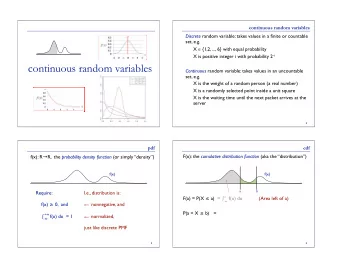
Continuous Random Variables Recall that when a random variable takes - PowerPoint PPT Presentation

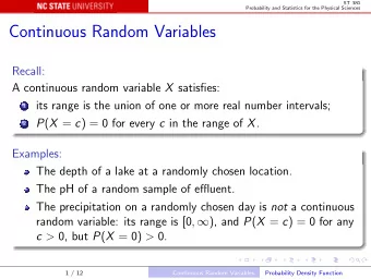
ST 370 Probability and Statistics for Engineers Continuous Random Variables Recall that when a random variable takes values in an entire interval, the variable is called continuous . Example: Flash unit recharge time The time that a flash unit takes to recharge could be any positive real number, in the interval (0 , ∞ ). 1 / 19 Continuous Random Variables Probability Density Functions

ST 370 Probability and Statistics for Engineers Probability Density Functions Suppose that we measure a random quantity X like a recharge time, but only to limited precision (such as to a certain number of decimal places), with values x 1 , x 2 , ... With no decimal places, x 1 = 0, x 2 = 1, ... With one decimal place, x 1 = 0 . 0, x 2 = 0 . 1, ... Then the measured variable Y is discrete, with a probability mass function f Y ( x i ) = P ( Y = x i ) . 2 / 19 Continuous Random Variables Probability Density Functions

ST 370 Probability and Statistics for Engineers Suppose that the probability mass function of Y can be approximated by a smooth function f X ( x ): f Y ( x i ) ≈ δ x f X ( x i ) , where δ x is the spacing of the x i . The cumulative distribution function of Y is � F Y ( x ) = f Y ( x i ) x i ≤ x � ≈ δ x f X ( x i ) x i ≤ x � x f X ( u ) du . ≈ −∞ 3 / 19 Continuous Random Variables Probability Density Functions

ST 370 Probability and Statistics for Engineers As δ x is made smaller, Y becomes a better approximation to X , and F X ( x ) = P ( X ≤ x ) = lim δ x → 0 P ( Y ≤ x ) � x = f X ( u ) du . −∞ 4 / 19 Continuous Random Variables Probability Density Functions

ST 370 Probability and Statistics for Engineers The smooth function f X ( x ) is the probability density function (pdf) of X . Probability density functions have the properties: f X ( x ) ≥ 0; � ∞ −∞ f X ( x ) dx = 1; � b P ( a ≤ X ≤ b ) = a f X ( x ) dx . Any function with the first two properties could be the probability density function of some random variable X . By the fundamental theorem of calculus, � x f X ( u ) du ⇒ f X ( x ) = dF X ( x ) F X ( x ) = . dx −∞ 5 / 19 Continuous Random Variables Probability Density Functions

ST 370 Probability and Statistics for Engineers Expected Value and Variance Just as the cumulative distribution function is: a sum for a discrete random variable; an integral for a continuous random variable, the expected value of a continuous random variable is an integral: � ∞ µ X = E ( X ) = xf X ( x ) dx . −∞ Similarly for the variance � ∞ σ 2 ( x − µ X ) 2 f X ( x ) dx . X = V ( X ) = −∞ 6 / 19 Continuous Random Variables Expected Value and Variance

ST 370 Probability and Statistics for Engineers Expected value of a function of X If Z = h ( X ) is a function of the random variable X , then Z is also a random variable, with expected value � ∞ E ( Z ) = E [ h ( X )] = h ( x ) f X ( x ) dx . −∞ Note that in general E [ h ( X )] � = h [ E ( X )] , except in the special case of a linear function h ( x ) = ax + b : E ( aX + b ) = aE ( X ) + b , which follows from the properties of integrals (and sums). 7 / 19 Continuous Random Variables Expected Value and Variance

ST 370 Probability and Statistics for Engineers Continuous Uniform Distribution The simplest probability density function is that of the continuous uniform distribution, which is a constant over some interval [ a , b ]: � 1 a ≤ x ≤ b b − a f ( x ) = 0 otherwise . R graphs x <- c(-1, 0, 0, 0, 1, 1, 1, 2); pdf <- c(0, 0, NA, 1, 1, NA, 0, 0); cdf <- c(0, 0, 0, 0, 1, 1, 1, 1); par(mfrow = c(2, 1)); plot(x, pdf, type = "l"); plot(x, cdf, type = "l") 8 / 19 Continuous Random Variables Continuous Uniform Distribution

ST 370 Probability and Statistics for Engineers Expected value: � b b � x 2 1 1 �� = a + b � E ( X ) = b − ax dx = . � b − a 2 2 � a a Variance: � b b − a ( x − µ X ) 2 dx = ( b − a ) 2 1 V ( X ) = . 12 a 9 / 19 Continuous Random Variables Continuous Uniform Distribution

ST 370 Probability and Statistics for Engineers The special case a = 0, b = 1 plays a central role in simulation of random variables. If U is uniformly distributed on [0 , 1] and F X ( x ) is any cumulative distribution function, then the random variable X = F − 1 X ( U ) has that cumulative distribution function. So if we have a mechanism for simulating U (such as a pseudo-random number generator), and we can efficiently calculate F − 1 X ( u ), we can simulate variables with any distribution (continuous or discrete). 10 / 19 Continuous Random Variables Continuous Uniform Distribution

ST 370 Probability and Statistics for Engineers Exponential Distribution The exponential distribution has the probability density function � λ e − λ x x ≥ 0 , f ( x ) = 0 x < 0 . and cumulative distribution function � x  λ e − λ u du = 1 − e − λ x x ≥ 0 ,  F ( x ) = 0 0 x < 0 .  It is the continuous analog of the geometric distribution. 11 / 19 Continuous Random Variables Exponential Distribution

ST 370 Probability and Statistics for Engineers R graphs x <- c(-1, -0.001, NA, seq(from = 0, to = 3, length = 101)); pdf <- dexp(x); cdf <- pexp(x); par(mfrow = c(2, 1)); plot(x, pdf, type = "l"); plot(x, cdf, type = "l") 12 / 19 Continuous Random Variables Exponential Distribution

ST 370 Probability and Statistics for Engineers Note that F − 1 ( u ) = − 1 λ log(1 − u ) so we can simulate an exponentially distributed random variable as X = − 1 λ log(1 − U ) where U has the uniform distribution on [0 , 1]. Since V = 1 − U is also uniformly distributed on [0 , 1], we could write this more simply as X = − 1 λ log( V ) . 13 / 19 Continuous Random Variables Exponential Distribution

ST 370 Probability and Statistics for Engineers Expected value: � ∞ x λ e − λ x dx = 1 E ( X ) = λ 0 Variance: � ∞ ( x − λ ) 2 λ e − λ x dx = 1 V ( X ) = λ 2 0 14 / 19 Continuous Random Variables Exponential Distribution

ST 370 Probability and Statistics for Engineers Poisson process The Poisson process is a model for points distributed randomly on a line, such as the arrival times of customers in a queuing model. It is characterized by the properties: The number of points that appear in an interval of length T has the Poisson distribution with parameter θ = λ T for some rate constant λ > 0; The numbers of points appearing in disjoint intervals are independent of each other. 15 / 19 Continuous Random Variables Exponential Distribution

ST 370 Probability and Statistics for Engineers Let X be the time of the first arrival. Then F X ( x ) = P ( X ≤ x ) = 1 − P ( X > x ) = 1 − P (no points in [0 , x ]) = 1 − e − λ x So X is exponentially distributed with parameter λ ; we can also show that the time from any arrival to the next arrival is exponentially distributed, with the same parameter. The exponential distribution is often used to model inter-arrival times of events like customer arrivals, major oil spills, shipping accidents, and many others. 16 / 19 Continuous Random Variables Exponential Distribution

ST 370 Probability and Statistics for Engineers Gamma Distribution The probability density function of the Gamma distribution is f ( x ) = λ r x r − 1 e − λ x x > 0 Γ( r ) where Γ( r ) is the gamma function, and λ > 0 and r > 0 are parameters of the distribution. If r is an integer, the waiting time until the r th event in a Poisson process has this distribution, which in this case ( r an integer) is called the Erlang distribution. The exponential distribution is the special case r = 1. 17 / 19 Continuous Random Variables Gamma Distribution

ST 370 Probability and Statistics for Engineers Expected value: E ( X ) = r λ Variance: V ( X ) = r λ 2 The Gamma distribution is the continuous time analog of the negative binomial distribution. 18 / 19 Continuous Random Variables Gamma Distribution

ST 370 Probability and Statistics for Engineers Weibull Distribution Another family that generalizes the exponential distribution is the Weibull distribution family, often used in reliability theory to model time to failure of some item or piece of equipment. The probability density function is complicated, as are the formulas for the expected value and variance. The properties of a Weibull random variable can be derived from the fact that, if X has the standard exponential distribution, and δ and β are positive, then W = δ × X 1 /β has a Weibull distribution. So if β = 1, X is an exponentially distributed random variable, and, if β � = 1, X is some positive power of an exponentially distributed random variable. 19 / 19 Continuous Random Variables Weibull Distribution