Continuous Expectation and Variance, the Law of Large Numbers, and - PowerPoint PPT Presentation

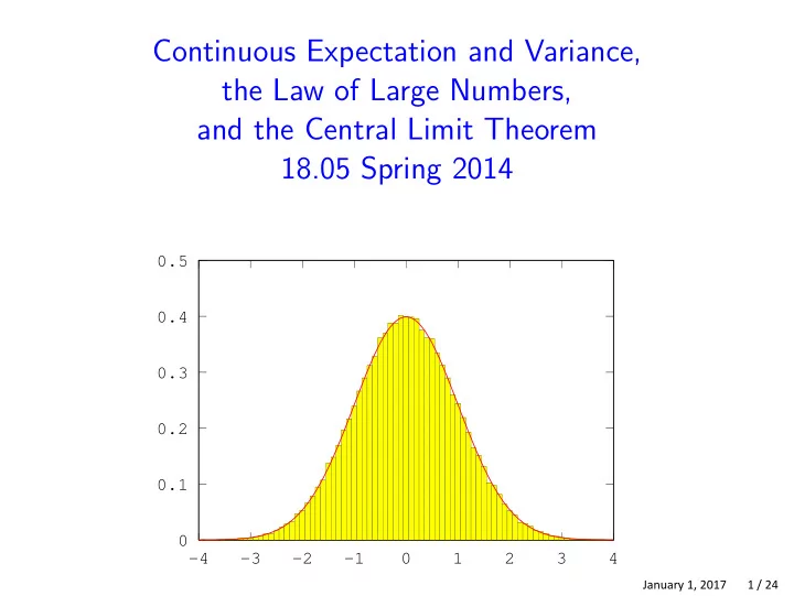
Continuous Expectation and Variance, the Law of Large Numbers, and the Central Limit Theorem 18.05 Spring 2014 0.5 0.4 0.3 0.2 0.1 0 -4 -3 -2 -1 0 1 2 3 4 January 1, 2017 1 / 24

Expected value Expected value: measure of location, central tendency X continuous with range [ a , b ] and pdf f ( x ): � b E ( X ) = xf ( x ) dx . a X discrete with values x 1 , . . . , x n and pmf p ( x i ): n n E ( X ) = x i p ( x i ) . i =1 View these as essentially the same formulas. January 1, 2017 2 / 24

Variance and standard deviation Standard deviation: measure of spread, scale For any random variable X with mean µ Var( X ) = E (( X − µ ) 2 ) , σ = Var( X ) X continuous with range [ a , b ] and pdf f ( x ): b � ( x − µ ) 2 f ( x ) dx . Var( X ) = a X discrete with values x 1 , . . . , x n and pmf p ( x i ): n n ( x i − µ ) 2 p ( x i ) . Var( X ) = i =1 View these as essentially the same formulas. January 1, 2017 3 / 24

Properties Properties: (the same for discrete and continuous) 1. E ( X + Y ) = E ( X ) + E ( Y ). 2. E ( aX + b ) = aE ( X ) + b . 3. If X and Y are independent then Var( X + Y ) = Var( X ) + Var( Y ). 4. Var( aX + b ) = a 2 Var( X ). 2 ) − E ( X ) 2 . 5. Var( X ) = E ( X January 1, 2017 4 / 24

Board question 2 The random variable X has range [0,1] and pdf cx . (a) Find c . (b) Find the mean, variance and standard deviation of X . (c) Find the median value of X . (d) Suppose X 1 , . . . X 16 are independent identically-distributed copies of X . Let X be their average. What is the standard deviation of X ? 4 . Find the pdf of Y . (e) Suppose Y = X January 1, 2017 5 / 24

Quantiles Quantiles give a measure of location. φ ( z ) left tail area = prob. = .6 z q 0 . 6 = 0 . 253 Φ( z ) 1 F ( q 0 . 6 ) = 0 . 6 z q 0 . 6 = 0 . 253 q 0 . 6 : left tail area = 0.6 ⇔ F ( q 0 . 6 ) = 0 . 6 January 1, 2017 6 / 24

Concept question Each of the curves is the density for a given random variable. The median of the black plot is always at q . Which density has the greatest median? 1. Black 2. Red 3. Blue 4. All the same 5. Impossible to tell (A) (B) Curves coincide to here. q q January 1, 2017 7 / 24

Law of Large Numbers (LoLN) Informally: An average of many measurements is more accurate than a single measurement. Formally: Let X 1 , X 2 , . . . be i.i.d. random variables all with mean µ and standard deviation σ . Let n X 1 + X 2 + . . . + X n 1 n X n = = X i . n n i =1 Then for any (small number) a , we have lim P ( | X n − µ | < a ) = 1 . n →∞ No guarantees but: By choosing n large enough we can make X n as close as we want to µ with probability close to 1. January 1, 2017 8 / 24

Concept Question: Desperation You have $100. You need $1000 by tomorrow morning. Your only way to get it is to gamble. If you bet $k, you either win $k with probability p or lose $k with probability 1 − p . Maximal strategy: Bet as much as you can, up to what you need, each time. Minimal strategy: Make a small bet, say $5, each time. 1. If p = 0 . 45, which is the better strategy? (a) Maximal (b) Minimal (c) They are the same 2. If p = 0 . 8, which is the better strategy? (a) Maximal (b) Minimal (c) They are the same January 1, 2017 9 / 24

Histograms Made by ‘binning’ data. Frequency : height of bar over bin = number of data points in bin. Density : area of bar is the fraction of all data points that lie in the bin. So, total area is 1. frequency density 4 0.8 3 0.6 2 0.4 1 0.2 x x 0.25 0.75 1.25 1.75 2.25 0.25 0.75 1.25 1.75 2.25 Check that the total area of the histogram on the right is 1. January 1, 2017 10 / 24

Board question 1. Make both a frequency and density histogram from the data below. Use bins of width 0.5 starting at 0. The bins should be right closed. 1 1.2 1.3 1.6 1.6 2.1 2.2 2.6 2.7 3.1 3.2 3.4 3.8 3.9 3.9 2. Same question using unequal width bins with edges 0, 1, 3, 4. 3. For question 2, why does the density histogram give a more reasonable representation of the data. January 1, 2017 11 / 24

Solution 3.0 0.4 Frequency Density 2.0 0.2 1.0 0.0 0.0 0 1 2 3 4 0 1 2 3 4 Histograms with equal width bins 0.4 8 Frequency Density 6 0.2 4 2 0.0 0 0 1 2 3 4 0 1 2 3 4 Histograms with unequal width bins January 1, 2017 12 / 24

LoLN and histograms LoLN implies density histogram converges to pdf: 0.5 0.4 0.3 0.2 0.1 0 -4 -3 -2 -1 0 1 2 3 4 Histogram with bin width 0.1 showing 100000 draws from a standard normal distribution. Standard normal pdf is overlaid in red. January 1, 2017 13 / 24

Standardization Random variable X with mean µ and standard deviation σ . X − µ Standardization: Y = . σ Y has mean 0 and standard deviation 1. Standardizing any normal random variable produces the standard normal. If X ≈ normal then standardized X ≈ stand. normal. We use reserve Z to mean a standard normal random variable. January 1, 2017 14 / 24

Concept Question: Standard Normal within 1 · σ ≈ 68% Normal PDF within 2 · σ ≈ 95% within 3 · σ ≈ 99% 68% 95% 99% z − σ σ − 3 σ − 2 σ 2 σ 3 σ 1 . P ( − 1 < Z < 1) is (a) 0.025 (b) 0.16 (c) 0.68 (d) 0.84 (e) 0.95 2. P ( Z > 2) (a) 0.025 (b) 0.16 (c) 0.68 (d) 0.84 (e) 0.95 January 1, 2017 15 / 24

Central Limit Theorem Setting: X 1 , X 2 , . . . i.i.d. with mean µ and standard dev. σ . For each n : 1 X n = ( X 1 + X 2 + . . . + X n ) average n S n = X 1 + X 2 + . . . + X n sum . Conclusion: For large n : � σ 2 � X n ≈ N µ, n S n ≈ N n µ, n σ 2 Standardized S n or X n ≈ N(0 , 1) S n − n µ X n − µ √ √ That is, = ≈ N(0 , 1) . n σ σ/ n January 1, 2017 16 / 24

CLT: pictures Standardized average of n i.i.d. uniform random variables with n = 1 , 2 , 4 , 12. 0.4 0.5 0.35 0.4 0.3 0.25 0.3 0.2 0.2 0.15 0.1 0.1 0.05 0 0 -3 -2 -1 0 1 2 3 -3 -2 -1 0 1 2 3 0.4 0.4 0.35 0.35 0.3 0.3 0.25 0.25 0.2 0.2 0.15 0.15 0.1 0.1 0.05 0.05 0 0 -3 -2 -1 0 1 2 3 -3 -2 -1 0 1 2 3 January 1, 2017 17 / 24

CLT: pictures 2 The standardized average of n i.i.d. exponential random variables with n = 1 , 2 , 8 , 64. 1 0.7 0.6 0.8 0.5 0.6 0.4 0.3 0.4 0.2 0.2 0.1 0 0 -3 -2 -1 0 1 2 3 -3 -2 -1 0 1 2 3 0.5 0.5 0.4 0.4 0.3 0.3 0.2 0.2 0.1 0.1 0 0 -3 -2 -1 0 1 2 3 -3 -2 -1 0 1 2 3 January 1, 2017 18 / 24

CLT: pictures 3 The standardized average of n i.i.d. Bernoulli(0.5) random variables with n = 1 , 2 , 12 , 64. 0.4 0.4 0.35 0.35 0.3 0.3 0.25 0.25 0.2 0.2 0.15 0.15 0.1 0.1 0.05 0.05 0 0 -3 -2 -1 0 1 2 3 -3 -2 -1 0 1 2 3 0.4 0.4 0.35 0.35 0.3 0.3 0.25 0.25 0.2 0.2 0.15 0.15 0.1 0.1 0.05 0.05 0 0 -3 -2 -1 0 1 2 3 -4 -3 -2 -1 0 1 2 3 4 January 1, 2017 19 / 24

CLT: pictures 4 The (non-standardized) average of n Bernoulli(0.5) random variables, with n = 4 , 12 , 64. (Spikier.) 1.4 3 1.2 2.5 1 2 0.8 1.5 0.6 1 0.4 0.5 0.2 0 0 -1 -0.5 0 0.5 1 1.5 2 -0.2 0 0.2 0.4 0.6 0.8 1 1.2 1.4 7 6 5 4 3 2 1 0 -0.2 0 0.2 0.4 0.6 0.8 1 1.2 1.4 January 1, 2017 20 / 24

Table Question: Sampling from the standard normal distribution As a table, produce a single random sample from (an approximate) standard normal distribution. The table is allowed nine rolls of the 10-sided die. Note: µ = 5 . 5 and σ 2 = 8 . 25 for a single 10-sided die. Hint: CLT is about averages. January 1, 2017 21 / 24

Board Question: CLT 1. Carefully write the statement of the central limit theorem. 2. To head the newly formed US Dept. of Statistics, suppose that 50% of the population supports Ani, 25% supports Ruthi, and the remaining 25% is split evenly between Efrat, Elan, David and Jerry. A poll asks 400 random people who they support. What is the probability that at least 55% of those polled prefer Ani? 3. What is the probability that less than 20% of those polled prefer Ruthi? January 1, 2017 22 / 24

Bonus problem Not for class. Solution will be posted with the slides. An accountant rounds to the nearest dollar. We’ll assume the error in rounding is uniform on [-0.5, 0.5]. Estimate the probability that the total error in 300 entries is more than $5. January 1, 2017 23 / 24

MIT OpenCourseWare https://ocw.mit.edu 18.05 Introduction to Probability and Statistics Spring 2014 For information about citing these materials or our Terms of Use, visit: https://ocw.mit.edu/terms.