Context-specific independence Parameter learning: MLE Graphical - PowerPoint PPT Presentation

Use Chapter 3 of K&F as a reference for CSI Reading for parameter learning: Chapter 12 of K&F Context-specific independence Parameter learning: MLE Graphical Models – 10708 Carlos Guestrin Carnegie Mellon University October 5 th , 2005

Announcements � Homework 2: � Out today/tomorrow � Programming part in groups of 2-3 � Class project � Teams of 2-3 students � Ideas on the class webpage, but you can do your own � Timeline: � 10/19: 1 page project proposal � 11/14: 5 page progress report (20% of project grade) � 12/2: poster session (20% of project grade) � 12/5: 8 page paper (60% of project grade) � All write-ups in NIPS format (see class webpage)

Clique trees versus VE � Clique tree advantages � Multi-query settings � Incremental updates � Pre-computation makes complexity explicit � Clique tree disadvantages � Space requirements – no factors are “deleted” � Slower for single query � Local structure in factors may be lost when they are multiplied together into initial clique potential

Clique tree summary � Solve marginal queries for all variables in only twice the cost of query for one variable � Cliques correspond to maximal cliques in induced graph � Two message passing approaches � VE (the one that multiplies messages) � BP (the one that divides by old message) � Clique tree invariant � Clique tree potential is always the same � We are only reparameterizing clique potentials � Constructing clique tree for a BN � from elimination order � from triangulated (chordal) graph � Running time (only) exponential in size of largest clique � Solve exactly problems with thousands (or millions, or more) of variables, and cliques with tens of nodes (or less)

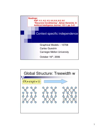
Global Structure: Treewidth w )) w exp( n ( O

Local Structure 1: Context specific indepencence Battery Age Alternator Fan Belt Charge Delivered Battery Fuel Pump Fuel Line Starter Distributor Gas Battery Power Spark Plugs Gas Gauge Engine Start Lights Engine Turn Over Radio

Local Structure 1: Context specific indepencence Context Specific I ndependence (CSI ) After observing a variable, some vars become independent Battery Age Alternator Fan Belt Charge Delivered Battery Fuel Pump Fuel Line Starter Distributor Gas Battery Power Spark Plugs Gas Gauge Engine Start Lights Engine Turn Over Radio

CSI example: Tree CPD Apply SAT Letter � Represent P(X i | Pa Xi ) using a decision tree � Path to leaf is an assignment to (a subset Job of) Pa Xi � Leaves are distributions over X i given assignment of Pa Xi on path to leaf � Interpretation of leaf : � For specific assignment of Pa Xi on path to this leaf – X i is independent of other parents � Representation can be exponentially smaller than equivalent table

Tabular VE with Tree CPDs � If we turn a tree CPD into table � “Sparsity” lost ! � Need inference approach that deals with tree CPD directly !

Local Structure 2: Determinism Determinism I f Battery Power = Dead , Battery Age Alternator Fan Belt then Lights = OFF Lights Charge Delivered Battery ON OFF Fuel Pump Fuel Line Battery OK .99 .01 Power Starter Distributor Gas .80 WEAK .20 Battery Power 0 1 DEAD Gas Gauge Spark Plugs Engine Start Lights Engine Turn Over Radio

Determinism and inference � Determinism gives a little Lights sparsity in table, but much ON OFF Battery bigger impact on inference OK .99 .01 Power .80 WEAK .20 � Multiplying deterministic factor 0 1 with other factor introduces DEAD many new zeros � Operations related to theorem proving, e.g., unit resolution

Today’s Models … � Often characterized by: � Richness in local structure (determinism, CSI) � Massiveness in size (10,000’s variables) � High connectivity (treewidth) � Enabled by: � High level modeling tools: relational, first order � Advances in machine learning � New application areas (synthesis): � Bioinformatics (e.g. linkage analysis) � Sensor networks � Exploiting local structure a must!

Exact inference in large models is possible… � BN from a relational model

Recursive Conditioning � Treewidth complexity (worst case) � Better than treewidth complexity with local structure � Provides a framework for time-space tradeoffs � Only quick intuition today, details: � Koller&Friedman: 3.1-3.4, 6.4-6.6 � “Recursive Conditioning”, Adnan Darwiche. In Artificial Intelligence Journal, 125:1, pages 5-41

The Computational Power of Assumptions Alternator Fan Belt Battery Age Leak Charge Delivered Battery Fuel Line Starter Gas Distributor Battery Power Spark Plugs Gas Gauge Engine Start Lights Engine Turn Over Radio A. Darwiche

The Computational Power of Assumptions Alternator Fan Belt Battery Age Leak Charge Delivered Battery Fuel Line Starter Gas Distributor Battery Power Spark Plugs Gas Gauge Engine Start Lights Engine Turn Over Radio A. Darwiche

Decomposition Alternator Fan Belt Battery Age Leak Charge Delivered Battery Fuel Line Starter Gas Distributor Battery Power Spark Plugs Gas Gauge Engine Start Lights Engine Turn Over Radio A. Darwiche

Case Analysis Battery Age Alternator Fan Belt Battery Age Alternator Fan Belt Leak Leak Charge Delivered Charge Delivered Battery Fuel Line Battery Fuel Line Starter Gas Starter Distributor Gas Distributor Battery Power Battery Power Spark Plugs Spark Plugs Gas Gauge Gas Gauge Lights Engine Turn Over Engine Start Radio Lights Engine Turn Over Engine Start Radio + p p A. Darwiche

Case Analysis Battery Age Alternator Fan Belt Battery Age Alternator Fan Belt Leak Leak Charge Delivered Charge Delivered Battery Fuel Line Battery Fuel Line Starter Gas Starter Distributor Gas Distributor Battery Power Battery Power Spark Plugs Spark Plugs Gas Gauge Gas Gauge Lights Engine Turn Over Engine Start Radio Lights Engine Turn Over Engine Start Radio * + p l p r p A. Darwiche

Case Analysis Battery Age Alternator Fan Belt Battery Age Alternator Fan Belt Leak Leak Charge Delivered Charge Delivered Battery Fuel Line Battery Fuel Line Starter Gas Starter Distributor Gas Distributor Battery Power Battery Power Spark Plugs Spark Plugs Gas Gauge Gas Gauge Lights Engine Turn Over Engine Start Radio Lights Engine Turn Over Engine Start Radio * + * p l p r p l p r A. Darwiche

Case Analysis Alternator Fan Belt Battery Age Battery Age Alternator Fan Belt Leak Leak Charge Delivered Charge Delivered Battery Fuel Line Battery Fuel Line Starter Gas Starter Distributor Gas Distributor Battery Power Battery Power Spark Plugs Spark Plugs Gas Gauge Gas Gauge Lights Engine Turn Over Engine Start Radio Lights Engine Turn Over Engine Start Radio * + * p l p r p l p r A. Darwiche

Case Analysis Alternator Fan Belt Battery Age Battery Age Alternator Fan Belt Leak Leak Charge Delivered Charge Delivered Battery Fuel Line Battery Fuel Line Starter Gas Starter Distributor Gas Distributor Battery Power Battery Power Spark Plugs Spark Plugs Gas Gauge Gas Gauge Lights Engine Turn Over Engine Start Radio Lights Engine Turn Over Engine Start Radio * + * p l p r p l p r A. Darwiche

Decomposition Tree A B C D E Cutset B A B B C A f(A) f(B,C) f(A,B) B C D E D f(C,D) f(B,D,E) A. Darwiche

Decomposition Tree A B C D E Cutset B A B B C A f(A) f(B,C) f(A,B) B C D E D f(C,D) f(B,D,E) A. Darwiche

Decomposition Tree A B C D E Cutset B A B C A f(A) f(B,C) f(A,B) Time: O(n exp(w log n)) C D E Space: Linear D f(C,D) (using appropriate dtree) f(B,D,E) A. Darwiche

RC1 RC1(T,e) // compute probability of evidence e on dtree T If T is a leaf node Return Lookup(T,e) Else p := 0 for each instantiation c of cutset(T)-E do p := p + RC1(Tl,ec) RC1(Tr,ec) return p A. Darwiche

Lookup(T, e ) Θ X| U : CPT associated with leaf T If X is instantiated in e , then x: value of X in e u : value of U in e Return θ x| u Else return 1 = Σ x θ x| u A. Darwiche

Caching A B C D E F A B Context A C ABC C .27 ABC A B C ABC B A C .39 ABC B C ABC ABC C ABC D ABC E F D E A. Darwiche

Caching A B C D E F Recursive Conditioning A An any-space algorithm with treewidth complexity B Darwiche AIJ-01 Context A C ABC Time: O(n exp(w)) C .27 ABC Space: O(n exp(w)) A B C ABC B A C (using appropriate dtree) .39 ABC B C ABC ABC C ABC D ABC E F D E A. Darwiche

RC2 RC2(T, e ) If T is a leaf node, return Lookup(T,e) y := instantiation of context(T) If cache T [ y ] < > nil, return cache T [ y ] p := 0 For each instantiation c of cutset(T)- E do p := p + RC2(T l , ec ) RC2(T r , ec ) cache T [ y ] := p Return p A. Darwiche

Decomposition with Local Structure X I ndependent of B, C given A A, B, C A X B C A. Darwiche

Decomposition with Local Structure X I ndependent of B, C given A A, B, C A X B C A. Darwiche

Decomposition with Local Structure X I ndependent of B, C given A A, B, C No need to consider an exponential number of cases (in the cutset size) given local structure A X B C A. Darwiche