MLE, MAP, AND NAIVE BAYES 10-601 RECITATION MARY MCGLOHON MLE The - PowerPoint PPT Presentation

MLE, MAP, AND NAIVE BAYES 10-601 RECITATION MARY MCGLOHON

MLE The usual representation we come across is a P ( X = x | θ ) probability density function: x 1 , x 2 , ..., x n ∼ N ( µ, σ 2 ) But what if we know that , but we don’t know ? µ P ( x | µ, σ ) We can set up a likelihood equation: , and find the value of that maximizes it. µ

MLE OF MU Since x’s are independent and from the same n distribution, � p ( x | µ, σ 2 ) = p ( x i | µ, σ 2 ) i =1 n n - exp (( x i − µ ) 2 1 � � p ( x i | µ, σ 2 ) = √ L ( x ) = ) 2 σ 2 2 πσ 2 i =1 i =1 Taking the log likelihood (we get to do this since log is monotonic) and removing some constants: n 2 � log ( L ( x )) = l ( x ) ∝ − ( x i − µ ) i =1

CALCULUS! We can take the derivative of this value and set it equal to zero, to maximize. n n dl ( x ) = d � � x 2 i − x i µ + µ 2 ) = − dx ( − x i − µ dx i =1 i =1 n n � n i =1 x i � � x i − µ = 0 → nµ = x i → µ = − n i =1 i =1

ABOUT THE MLE We can’t always do this analytically, but there are all sorts of tricks. (See homework). This is the traditional statistical approach to finding parameters. (The Unbiased M.L.E.)

ABOUT THE MLE We can’t always do this analytically, but there are all sorts of tricks. (See homework). This is the traditional statistical approach to finding parameters. (The Unbiased M.L.E.)

MAP What if you have some ideas about your parameter? In the Bayesian school of thought (or “cult”, depending on who you ask)... We can use Bayes’ Rule: P ( θ | x ) = P ( x | θ ) P ( θ ) = P ( x | θ ) P ( θ ) P ( x | θ ) P ( θ ) Θ P ( θ , x ) = P ( x ) � � Θ P ( x | θ ) P ( θ )

MAP P ( x | θ ) P ( θ ) argmax θ P ( θ | x ) = argmax θ � Θ P ( x | θ ) P ( θ ) This is just maximizing the numerator, since the denominator is a normalizing constant. (Emcee M.C.) This assumes a prior distribution, . P ( θ ) Old-school statisticians hate that. But if you get a good estimate of the prior, you’ll probably be ok. (This is why we don’t have old-school statisticians writing spam filters.)

MAP P ( x | θ ) P ( θ ) argmax θ P ( θ | x ) = argmax θ � Θ P ( x | θ ) P ( θ ) This is just maximizing the numerator, since the denominator is a normalizing constant. (Emcee M.C.) This assumes a prior distribution, . P ( θ ) Old-school statisticians hate that. But if you get a good estimate of the prior, you’ll probably be ok. (This is why we don’t have old-school statisticians writing spam filters.)

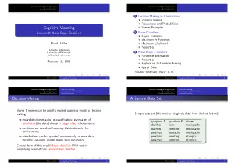
WHAT WE CAN DO NOW MAP is the foundation for Naive Bayes classifiers. Here, we’re assuming our data are drawn from two “classes”. We have a bunch of data where we know the class, and want to be able to predict P(class|data-point). So, we use empirical probabilities prediction = argmax C P ( C = c | X = x ) ∝ argmax C ˆ P ( X = x | C = c ) ˆ P ( C = c ) In NB, we also make the assumption that the features are conditionally independent .

SPAM FILTERING Suppose we wanted to build a spam filter. To use the “bag of words” approach, assuming that n words in an email are conditionally independent, we’d get: n ^ ^ � P ( spam | w ) ∝ P ( w i | spam ) P ( spam ) i =1 n ^ ^ � P ( ¬ spam | w ) ∝ P ( w i |¬ spam ) P ( ¬ spam ) i =1 Whichever one’s bigger wins!

THE IMPORTANCE OF THE SAMPLE What happens if you train on a set of data that’s mostly spam, and test on a set that’s mostly good emails? n ^ ^ � P ( spam | w ) ∝ P ( w i | spam ) P ( spam ) i =1 Also, just choosing one test set “wastes data”. What can we do?

CROSS-VALIDATION Cross-validation involves training several times. LOOCV (Leave-one-out cross validation): For each data point, train classifier on -- that is, x − i all data points besides , and classify . x i x i Error is the average accuracy. What’s wrong with this?

K-FOLDS CV A cheaper way of doing cross-validation is to divide (“fold”) the dataset into k pieces. For each piece i , Train on all data not in set i , classify set i . Report mean error. This is a “happy medium” between straight-up training/ testing and LOOCV.

LESS-NAIVE BAYES How would we modify NB to use two dependent attributes? P ( x i | c ) = P ( x i, 1 , x i, 2 , ..., x i,A | c ) Hint: -- you’re estimating the joint conditional distribution of the attributes.

CONTINUOUSLY NAIVE BAYES How could we modify NB for continuous attributes? For instance, classify whether you like basketball given your age (real), height (real), whether you like football (binary), and type of shoes you wear (categorical).

TOPOLOGY OF NAIVE BAYES What’s the decision surface for Naive Bayes? Hint: P ( c | word ) = P ( word | c ) I ( word ) + P ( ¬ word | c ) I ( ¬ word )