Construction of Manifolds via Compatible Sparse Representations - PowerPoint PPT Presentation
Construction of Manifolds via Compatible Sparse Representations Ruimin Wang, Ligang Liu , Zhouwang Yang, Kang Wang, Wen Shan, Jiansong Deng, Falai Chen University of Science and Technology of China Problem: Fitting Data with Smooth Surface
Construction of Manifolds via Compatible Sparse Representations Ruimin Wang, Ligang Liu , Zhouwang Yang, Kang Wang, Wen Shan, Jiansong Deng, Falai Chen University of Science and Technology of China
Problem: Fitting Data with Smooth Surface Point Cloud A Smooth Surface
Problem: Fitting Data with Smooth Surface • Challenging: capturing sharp features
Problem: Data Fitting • Input: A set of points 𝑦 𝑗 , 𝑧 𝑗 , 𝑗 = 0, … , 𝑜 • Output: A function which fits the point set 𝑧 = 𝑔 ( 𝑦 ) ( 𝑦 𝑜 , 𝑧 𝑜 ) ( 𝑦 𝑗 , 𝑧 𝑗 ) ( 𝑦 0 , 𝑧 0 )
Data Fitting: What Function? • What type of functions for 𝑔 ( 𝑦 ) ? 𝑧 = 𝑔 ( 𝑦 ) ( 𝑦 𝑜 , 𝑧 𝑜 ) ( 𝑦 𝑗 , 𝑧 𝑗 ) ( 𝑦 0 , 𝑧 0 )
Data Fitting: Function Space • Assuming: basis functions { 𝑐 𝑗 𝑦 , 𝑗 = 0, … , 𝑛 } • Finding a member in a family of functions: 𝑛 𝑔 ( 𝑦 ) = � 𝛽 𝑗 𝑐 𝑗 ( 𝑦 ) 𝑙=0 i.e., representing 𝑔 ( 𝑦 ) as a (coefficient) point 𝛽 = ( 𝛽 0 , 𝛽 1 ,…, 𝛽 𝑛 ) in 𝑆 𝑛+1 • Finding optimal ( 𝛽 0 , 𝛽 1 ,…, 𝛽 𝑛 ) by minimizing the fitting error: 𝛽 ( 𝑧 𝑗 − 𝑔 ( 𝑦 𝑗 )) 2 min
Data Fitting: Function Space • Basis functions { 𝑐 𝑗 𝑦 , 𝑗 = 0, … , 𝑛 } – Polynomial function basis {1, 𝑦 , 𝑦 2 , … , 𝑦 𝑛 } – Trigonometric function basis {1, sin 𝑦 , cos 𝑦 , sin 2𝑦 , cos 2𝑦 , … } – Exponential function basis {1, 𝑓 𝑦 , 𝑓 2𝑦 , … , 𝑓 𝑛𝑦 } – … • If we choose enough number of basis ( 𝑛 = 𝑜 ) , the fitting error can be 0! – the fitting function 𝑔 ( 𝑦 ) is an interpolation
Overfitting Problem • How to choose appropriate number of basis? 𝛽 0 + 𝛽 1 𝑦 + 𝛽 2 𝑦 2 + 𝛽 3 𝑦 3 + 𝛽 4 𝑦 4 𝛽 0 + 𝛽 1 𝑦 𝛽 0 + 𝛽 1 𝑦 + 𝛽 2 𝑦 2 High bias “Just right” High variance (underfitting) (overfitting)
Sparse Representation • An over-complete dictionary (atom functions) – Finding a ‘best’ fit from larger family of functions • Choose as least number of basis as possible – most of the elements of 𝛽 = ( 𝛽 0 , 𝛽 1 ,…, 𝛽 𝑛 ) are 0 – i.e., 𝛽 0 (number of non-zero elements) is less than some threshold 𝜀 𝛽 ( 𝑧 𝑗 − 𝑔 ( 𝑦 𝑗 )) 2 𝛽 ( 𝑧 𝑗 − 𝑔 ( 𝑦 𝑗 )) 2 min min s.t. 𝛽 0 ≤ 𝜀
3D Surface Case
Parameterization of Local Patch
Representing Sharp Features? • Smooth functions cannot represent 𝐷 0 sharp features cusp crease dart
Idea: 𝐷 0 Atom Functions • Introduce 𝐷 0 atom functions in the dictionary – Shape functions representing non-smooth finite elements in FEM • Each atom function – A bilinear quadrilateral element shape function defined on one edge A 𝐷 0 atom function defined on the edge (in red) of a vertex (in green) with valence 5
𝐷 0 Atom Functions • A total of 55 shape functions for vertices with valence 3-7 – Add more atom functions for vertices with valence > 7
Dictionary: Total Atom Functions • 120 polynomial functions with degree up to 14 • 55 𝐷 0 atom functions Underfitting Overfitting Result by A patch with sparse fitting sharp features
How to stitch local patches?
Manifold Representation
Previous Works on Manifold Construction • [Grimm and Hughes 1995] • [Ying and Zorin 2004] • [Gu et al. 2006] • [Wang et al. 2008] • [Della Vecchia and Juettler 2009] • [Tosun and Zorin 2011] • …
Application 1: Approximating Subdivision Surface
Problem • Construct manifolds to approximate subdivision surfaces with sharp features – Orange lines are specified as sharp features Input Mesh Manifold Surface
Construction of the Charts [Ying and Zorin 2004]
Incompatible Local Patches 𝑤 𝑗 𝑤 𝑘
Global Fitting Error
Global Fitting Error
Optimization Solver Forward error evaluation
Optimization Solver Forward error evaluation Backward Update
Optimization Solver Final Result Local sparse optimization and Global sparse optimization iteratively
Example Control mesh Result Top 5 selected atoms ( 𝐷 0 in red) Close-up
Different Subdivision Rules Control Mesh Different Geometry
More Examples
Application 2: Manifold from Curve Network
Sampling Points on Curves Input curve network Domain manifold Result manifold Sampled points Parameterization
Results Domain mesh Different manifold surfaces from different geometries
Results
Conclusions • A novel manifold construction method • Sparse representation for local geometry • Global compatibility • Representing sharp features
Future Work • No guarantee to capture all geometric features – Learning geometry features • Slow sparsity optimization – Speed up • Other applications – Surface reconstruction, denoising, and compression
Thank you! Ligang Liu, http://staff.ustc.edu.cn/~lgliu
Recommend
More recommend
Explore More Topics
Stay informed with curated content and fresh updates.
