Conditional Sampling for Max-Stable Random Fields Yizao Wang - - PowerPoint PPT Presentation

Conditional Sampling for Max-Stable Random Fields

Yizao Wang

Department of Statistics, the University of Michigan

June 28th, 2011 7th EVA Conference, Lyon, France Joint work with Stilian A. Stoev

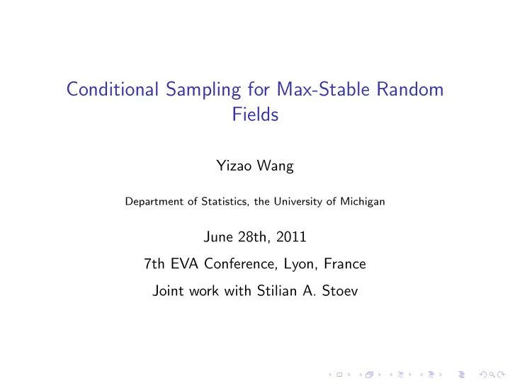
An Example

A sample from the Smith Model (Smith 1990): A stationary (moving maxima) max-stable random field.

−2 −1 1 −2 −1 1 2 4 6 8 10 12 2 2 2 2 2 4 4 4 4 4 6 6 6 8 8 1 1 12 2.97 0.74 0.86 3.83 9.67 0.89 7.8

If only partial observations (red crosses) are provided...

What We Can Do...

Four (fast) conditional samplings from the Smith Model:

−2 −1 1 −2 −1 1 2 4 6 8 10 12 2 2 2 2 2 4 4 4 4 4 6 6 6 8 8 10 1 12 2.97 0.74 0.86 3.83 9.67 0.89 7.8

−2 −1 1 −2 −1 1 2.97 0.74 0.86 3.83 9.67 0.89 7.8

2 2 2 2 4 4 4 4 6 6 6 6 8 8 8 10 10 12

−2 −1 1 −2 −1 1 2.97 0.74 0.86 3.83 9.67 0.89 7.8

2 2 2 4 4 4 6 6 6 8 8 10 10 12

−2 −1 1 −2 −1 1 2.97 0.74 0.86 3.83 9.67 0.89 7.8

2 2 2 2 4 4 4 6 6 6 8 8 10 10 12

−2 −1 1 −2 −1 1 2.97 0.74 0.86 3.83 9.67 0.89 7.8

2 2 2 2 2 4 4 6 6 6 8 8 8 10 10 12

2 4 6 8 10 12

◮ Potential applications in prediction. ◮ Analytical formula impossible in general. ◮ Need models with special structures.

Max-Linear Models

Definition

◮ Z1, . . . , Zp: iid α-Fr´

echet: P(Z > t) = exp{−σαt−α} .

◮ A = (ai,j) ∈ Rn×p +

given.

◮ Let X = A ⊙ Z denote

Xi =

p

• j=1

ai,jZj, i = 1, . . . , n . Remark

◮ {Xi}1≤i≤n is a spectrally discrete α-Fr´

echet process.

◮ Approximation of arbitrary max-stable process (random field)

with p sufficiently large.

◮ Results valid for non-negative Zj with densities fZj.

Conditional Sampling for Max-Linear Models

Our contribution: (W and Stoev 2011)

◮ Explicit formula of conditional distribution for max-linear

models (including a large class of max-stable random fields).

◮ Efficient algorithm (R package maxLinear) for large scale

conditional samplings.

◮ Potential applications in prediction for extremal phenomena,

e.g., environmental and financial problems. Two applications:

◮ MARMA processes (Davis and Resnick 1989, 1993). ◮ Smith model (Smith 1990).

MARMA Processes

Davis and Resnick (1989, 1993) Max-autoregressive moving average process (MARMA) (m, q): Xt = φ1Xt−1 ∨ · · · ∨ φmXt−m ∨ Zt ∨ θ1Zt−1 ∨ · · · ∨ θqZt−q , with t ∈ Z, φi ≥ 0, θj ≥ 0, {Zt}t∈Z iid 1-Fr´ echet. Or equivalently (iff φ∗ = m

i=1 φi < 1)

Xt =

∞

• j=0

ψjZt−j , t ∈ N with ψj ≥ 0, ∞

j=0 ψj < ∞ (explicit formula for ψj).

50 100 150 20 40 60 80 t X MARMA process Conditional 95% quantile Conditional median Projection predictor

Prediction of MARMA(3,0) processes

Prediction of a MARMA(3,0) process with φ1 = 0.7, φ2 = 0.5 and φ3 = 0.3, based on the observation of the first 100 values of the process.

Smith Model

A stationary max-stable random field model (Smith 1990): Xt =

• e

R2 φ(t − u)Mα(du),

t = (t1, t2) ∈ R2. with φ(t1, t2) := β1β2 2π

• 1 − ρ2 exp
• −

1 2(1 − ρ2)

• β2

1t2 1 − 2ρβ1β2t1t2 + β2 2t2 2

.

◮ Consistent estimators for ρ, β1, β2 (de Haan and Pereira 2006) ◮ A discretized version:

Xt =

• −q≤j1,j2≤q−1

h2/αφ(t − uj1j2)Zj1j2, t ∈ {−q, . . . , q}2 with uj1j2 = ((j1 + 1/2)h, (j2 + 1/2)h) and Zj1j2’s iid 1-Fr´ echet.

Simulations

−2 −1 1 −2 −1 1 5 5 5 5 5 5 5

5 5 5 5 10 10 15

−2 −1 1 −2 −1 1 5 5 5 5 5 5 5

5 5 5 5 5 1 1 15 15

−2 −1 1 −2 −1 1 5 5 5 5 5 5 5

2 2 2 4 4 4 4 6 6 6 6 6 8 8 8 1 12

−2 −1 1 −2 −1 1 5 5 5 5 5 5 5

2 4 4 4 4 6 6 6 8 8

5 10 15

Figure: 4 conditional samplings from Smith model. Parameters: ρ = 0, β1 = 1, β2 = 1 (isotropic).

Simulations

−2 −1 1 −2 −1 1 2 4 6 8 10 12 2 2 2 2 2 4 4 4 4 4 6 6 6 8 8 10 1 12 2.97 0.74 0.86 3.83 9.67 0.89 7.8 −2 −1 1 −2 −1 1 5 10 15 5 5 10 10 1 5 2.97 0.74 0.86 3.83 9.67 0.89 7.8

Figure: 95%-quantile of the conditional marginal deviation. Parameters: ρ = −0.8, β1 = 1.5, β2 = 0.7.

This Talk: an Inverse Problem and an Efficient Solution

−2 −1 1 −2 −1 1 5 5 5 5 5 5 5

5 5 5 5 10 10 15

−2 −1 1 −2 −1 1 5 5 5 5 5 5 5

5 5 5 5 5 1 1 15 15

−2 −1 1 −2 −1 1 5 5 5 5 5 5 5

2 2 2 4 4 4 4 6 6 6 6 6 8 8 8 1 12

−2 −1 1 −2 −1 1 5 5 5 5 5 5 5

2 4 4 4 4 6 6 6 8 8

5 10 15

Formulation of the Problem

◮ Random structures (models)

X = A ⊙ Z and Y = B ⊙ Z .

◮ Predict

P(Y ∈ · | X = x) .

◮ A ∈ Rn,p +

and B ∈ RnB,p

+

known.

◮ Key: conditional distribution

P(Z ∈ E | X = x) =? Remark

◮ Theoretical issue: P(Z ∈ E|X = x) is not well defined.

Rigorous treatment: regular conditional probability.

◮ Computational issue: n small, p, nB large.

A Toy Example

X1 = Z1 ∨ Z2 ∨ Z3 X2 = Z1 A = 1 1 1 1

• .

(In)equality constraints on Z: Z1 = X2 =: z1 Z2 ≤ X1 =: z2 Z3 ≤ X1 =: z3 . Case 1: (red) If X1 = X2 = x, then Z1 = z1 , Z2 ≤ z2 , Z3 ≤ z3 . In this case, P(Z ∈ E | case 1 ) = δ

z1(π1(E)) 3

• j=2

P{Zj ∈ πj(E)|Zj < zj}.

A Toy Example

X1 = Z1 ∨ Z2 ∨ Z3 X2 = Z1 A = 1 1 1 1

• .

(In)equality constraints on Z: Z1 = X2 =: z1 Z2 ≤ X1 =: z2 Z3 ≤ X1 =: z3 . Case 2: (blue) If x2 = X2 < X1 = x1, then Z1 = z1, and either Z1 = z1 , Z2 = z2 , Z3 ≤ z3

• r

Z1 = z1 , Z2 ≤ z2 , Z3 = z3 . In the first case (similar for the second), P(Z ∈ E | case 2 first ) =

2

• j=1

δ

zj(πj(E))P{Z3 ∈ π3(E)|Z3 <

z3}.

Observations from the Toy Example

We have seen...

◮ There are subcases that the conditional distributions are easy. ◮ The subcases are determined by the equality constraints.

It turns out...

◮ The desired conditional distribution is a mixture of the ones in

the subcases. An inverse problem

◮ Find all combinations of equality constraints that yield valid

subcases.

◮ Each subcase referred to as a hitting scenario J ⊂ {1, . . . , p}.

A Toy Example

X1 = Z1 ∨ Z2 ∨ Z3 X2 = Z1 . Case 1: (red) If X1 = X2 = x, then Z1 = z1 , Z2 < z2 , Z3 < z3 and J = {1} . Case 2: (blue) If x2 = X2 < X1 = x1, then Z1 = z1 , Z2 = z2 , Z3 < z3

• r

Z1 = z1 , Z2 < z2 , Z3 = z3 , and correspondingly, J = {1, 2} or J = {1, 3}. J = {3} is not a hitting scenario (and why?).

Hitting Scenarios

J ⊂ {1, . . . , p} is a hitting scenario, if CJ(A, x) ≡ {z ∈ Rp

+ : zj =

zj, j ∈ J, zk < zk, k ∈ Jc, A ⊙ z = x} is non-empty.

◮ Not every J ∈ {1, . . . , p} is a valid hitting scenario. ◮ Restricted to each CJ(A, x),

νJ(x, E) ≡ P(Z ∈ E | Z ∈ CJ(A, x)) =

• j∈J

δ

zj(πj(E))

• j∈Jc

P{Zj ∈ πj(E)|Zj < zj},

◮ {CJ(A, x)}J∈J mutually disjoint.

Conditional Distribution for Max-Linear Models

Theorem (W and Stoev 2011) P(Z ∈ E | X = x) is a mixture of νJ, indexed by J ∈ Jr(A, x). P(Z ∈ E | X = x) =

• J∈Jr(A,x)

pJ(A, x)νJ(x, E) , E ∈ RRp

+

where pJ(A, x) ∝ wJ :=

• j∈J
• zjfZj(

zj)

• j∈Jc

FZj( zj),

• J∈Jr(A,x)

pJ = 1 . Jr(A, x): all valid hitting scenarios.

Algorithm for conditional sampling Z | X = x

Algorithm I (1) compute z, Jr(A, x) and pJ(A, x), and (2) sample Z ∼ P(Z ∈ · | X = x). Not the end of the story!

◮ We haven’t discussed how to solve the inverse problem of

identification of Jr(A, x), which is closely related to the NP-hard set cover problem.

◮ Fortunately, by the max-linear structure, with probability 1,

Jr(A, x) has a nice structure, leading to an efficient algorithm.

An Efficient Algorithm in a Nut Shell

A standard algorithm takes exponentially long time to solve Jr(A, x) (and |Jr(A, x)| can be very large). But with probability 1,

◮ {1, . . . , p} = r s=1 J (s) (disjoint). ◮ Jr(A, x) determined by {J (s)}s=1,...,r:

Jr(A, x) = {J ⊂ {1, . . . , p} : |J ∩ J

(s)| = 1, s = 1, . . . , p} . ◮ Z can be divided into conditionally independent sub-vectors

{Zj}j∈J

(1), . . . , {Zj}j∈J (r) .

◮ {J (s)}s=1,...,r depending on (A, x) can be solved efficiently.

Factorization of Conditional Distribution Formula

Theorem (W and Stoev 2011) W.P.1, {1, . . . , p} = r

s=1 J (s) (mutually disjoint), and

ν(s)(x, ·) ≡ P({Zj}j∈J

(s) ∈ · | X = x)

has simple explicit formula. Algorithm II (thanks to the conditional independence) Z | X = x ← −      {Zj}j∈J

(1) | X = x ∼ ν(1)(x, ·)

· · · {Zj}j∈J

(r) | X = x ∼ ν(r)(x, ·)

Computational Efficiency

Time (in secs) of identification of {J

(s)}s=1,...,r for Algorithm II:

p \ n 1 5 10 50 2500 0.03 (0.02) 0.13 (0.03) 0.24 (0.04) 1.25 (0.09) 10000 0.11 (0.04) 0.50 (0.05) 1.00 (0.08) 4.98 (0.33) Comparison of two formulas:

• J∈Jr(A,x)

pJνJ(x, ·)

• Algorithm I

= ν(x, ·) =

r

• s=1

ν(s)(x, ·)

• Algorithm II

Summary

◮ Explicit formula of conditional distributions for max-linear

models (including a large class of max-stable random fields).

◮ Efficient algorithm (R package maxLinear) for large scale

conditional samplings. http://cran.r-project.org/web/packages/maxLinear/

◮ Future:

Potential applications in prediction for extremal phenomena, e.g., environmental and financial problems. Fitting A and B: a challenging problem.

References

Davis, R. A. and Resnick, S. I. (1989). Basic properties and prediction of max-ARMA processes.

• Adv. in Appl. Probab. 21, 781–803.

Davis, R. A. and Resnick, S. I. (1993). Prediction of stationary max-stable processes.

• Ann. Appl. Probab. 3, 497–525.

de Haan, L. (1984). A spectral representation for max-stable processes.

• Ann. Probab. 12, 1194–1204.

de Haan, L. and Pereira, T. T. (2006). Spatial extremes: Models for the stationary case. The Annals of Statistics 34, 146–168. Schlather, M. (2002). Models for stationary max–stable random fields. Extremes 5, 33–44.

References

Smith, R. L. (1990). Max–stable processes and spatial extremes. unpublished manuscript. Wang, Y. (2010). maxLinear: Conditional sampling for max-linear models. R package version 1.0. Wang, Y. and Stoev, S. A. (2011). Conditional sampling for spectrally discrete max-stable random fields.

• Adv. in Appl. Probab. 43, no. 2, 461–483.

Zhang, Z. and Smith, R. L. (2010). On the estimation and application of max-stable processes.

• J. Statist. Plann. Inference. 140 , no. 5, 1135–1153.

Auxiliary Results

Regular Conditional Probability

The regular conditional probability ν of Z given σ(X), is a function ν : Rn × BRp

+ → [0, 1] ,

such that (i) ν(x, ·) is a probability measure, for all x ∈ Rn, (ii) The function ν(·, E) is measurable, for all Borel sets E ∈ BRp. (iii) For all E ∈ RRp and D ∈ RRn, (PX(·) := P(X ∈ ·)): P(Z ∈ E, X ∈ D) =

• D

ν(x, E)PX(dx) . (1) We will first guess a formula for ν and then prove (1).

A Heuristic Proof

Consider a neighbor of CJ(A, x) (of P-measure 0) CJ(A, x) =

• z ∈ Rp

+ : zj =

zj, j ∈ J, zk < zk, k ∈ Jc C ǫ

J(A, x)

:=

• z ∈ Rp

+ : zj ∈ [

zj(1 − ǫ), zj(1 + ǫ)], j ∈ J, zk < zk(1 − ǫ) , k ∈ Jc for small enough ǫ > 0 and let C ǫ(A, x) :=

J∈J (A,x) C ǫ J(A, x).

The sets A ⊙ (C ǫ(A, x)) shrink to the point x, as ǫ ↓ 0. Proposition (W and Stoev 2010). For all x ∈ A ⊙ (Rp

+), we have,

as ǫ ↓ 0, P(Z ∈ E|Z ∈ C ǫ(A, x)) − → ν(x, E), ∀E ∈ RRp

+.

Remarks:

◮ Proved by Taylor expansion. ◮ The choice of C ǫ J(A, x) is delicate.

Set Cover Problem

◮ Let H = (hi,j)n×p with hi,j ∈ {0, 1}.

For example: H =   1 1 1 1 1 1   .

◮ Goal: use fewest columns to cover all rows (by ‘1’). Solutions

for the above problem: {1, 2}, {1, 3}, or {2, 3}.

◮ J ∈ Jr(A, x) 1−1

← → a solution of the hitting matrix H(A, x) defined by: hi,j = 1 iff Zj = zj yields Xi = xi .

◮ Set cover problem is NP-hard, but...

Simple Cases of Set Cover Problem

H1 =           1 1 1 1 1 1 1 1 1 1 1 1 1 1           , H2 =           1 1 1 1 1 1 1 1 1 1 1 1 1 1 1 1 1           . Two types of H:

◮ H1 hard: it takes a while to solve

r(J (H1)) = 4 and |Jr(H1)| = 6 .

◮ H2 nice: columns 1 and 5 are dominating. Therefore,

r(J (H2)) = 2 and J (H2) = {{1, 5}} . Lemma (W and Stoev 2011) W.p.1, H has nice structure.

When We Have Bad H? Another Toy Example

Consider X = A ⊙ Z with A =   2 1 1 1 1 1 2   . Different hitting matrices: Z1 > Z2, Z2 > 2Z3 ⇒ H =   1 1 1 1   Z1 < Z2 < 2Z1, Z2 > 2Z3 ⇒ H =   1 1 1 1   Z1 = Z2, Z2 > 2Z3 ⇒ H =   1 1 1 1 1  

Factorization of Regular Conditional Probability Formula

Theorem (W and Stoev 2011) With probability one, we have (i) for all J ⊂ [p], J ∈ Jr(A, A ⊙ Z) if and only if J can be written as J = {j1, . . . , jr} with js ∈ J(s) , ∀s ∈ [r] , (ii) For the regular conditional probability ν(x, E), ν(X, E) =

r

• s=1

ν(s)(X, E) with ν(s)(X, E) =

• j∈J(s) w(s)

j

ν(s)

j

(X, E)

• j∈J(s) w(s)

j

, where for all j ∈ J(s), w(s)

j

=

• zjfZj(

zj)

• k∈J

(s)\{j}

FZk( zk) ν(s)

j

(x, E) = δπj(E)( zj)

• k∈J

(s)\{j}

P(Zk ∈ πk(E)|Zk < zk) .