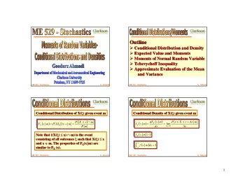
Conditional Random Fields [Hanna M. Wallach, Conditional Random - PDF document

Conditional Random Fields [Hanna M. Wallach, Conditional Random Fields: An Introduction, Technical Report MS-CIS- 04-21, University of Pensylvania, 2004 . ] CS 486/686 University of Waterloo Lecture 19: March 13, 2012 Outline • Conditional Random Fields 2 CS486/686 Lecture Slides (c) 2012 P. Poupart 1

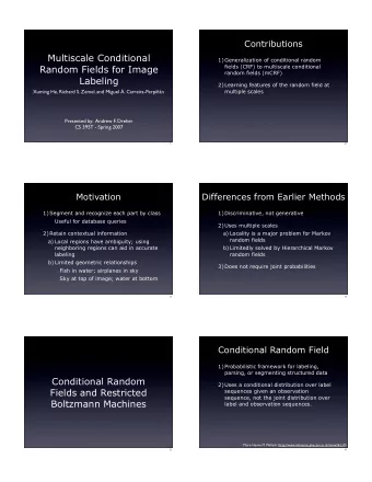
Conditional Random Fields • CRF: special Markov network that represents a conditional distribution • Pr( X | E ) = 1/k( E ) e  j  j  j ( X,E ) – NB: k( E ) is a normalization function (it is not a constant since it depends on E – see Slide 5) • Useful in classification: Pr(class|input) • Advantage: no need to model distribution over inputs 3 CS486/686 Lecture Slides (c) 2012 P. Poupart Conditional Random Fields • Joint distribution: – Pr( X,E ) = 1/k e  j  j  j ( X,E ) • Conditional distribution – Pr( X | E ) = e  j  j  j ( X,E ) /  X e  j  j  j ( X,E ) • Partition features in two sets: –  j1 ( X,E ): depend on at least one var in X –  j2 ( E ): depend only on evidence E 4 CS486/686 Lecture Slides (c) 2012 P. Poupart 2

Conditional Random Fields • Simplified conditional distribution: – Pr(X|E) = e  j1  j1  j1 ( X,E ) +  j2  j2  j2 ( E )  X e  j1  j1  j1 ( X,E ) +  j2  j2  j2 ( E ) = e  j1  j1  j1 ( X,E ) e  j2  j2  j2 ( E )  X e  j1  j1  j1 ( X,E ) e  j2  j2  j2 ( E ) = 1/k( E ) e  j1  j1  j1 ( X,E ) • Evidence features can be ignored! 5 CS486/686 Lecture Slides (c) 2012 P. Poupart Parameter Learning • Parameter learning is simplified since we don’t need to model a distribution over the evidence • Objective: maximum conditional likelihood –  * = argmax  P(X=x|  ,E=e) – Convex optimization, but no closed form – Use iterative technique (e.g., gradient descent) 6 CS486/686 Lecture Slides (c) 2012 P. Poupart 3

Sequence Labeling • Common task in – Entity recognition – Part of speech tagging – Robot localisation – Image segmentation • L* = argmax L Pr( L | O )? = argmax L 1 ,…,L n Pr(L 1 ,…,L n |O 1 ,…,O n )? 7 CS486/686 Lecture Slides (c) 2012 P. Poupart Hidden Markov Model S 1 S 2 S 3 S 4 O 1 O 2 O 3 O 4 • Assumption: observations are independent given the hidden state 8 CS486/686 Lecture Slides (c) 2012 P. Poupart 4

Conditional Random Fields • Since the distribution over observations is not modeled, there is no independence assumption among observations S 1 S 2 S 3 S 4 O 1 O 2 O 3 O 4 • Can also model long-range dependencies without significant computational cost 9 CS486/686 Lecture Slides (c) 2012 P. Poupart Entity Recognition • Task: label each word with a predefined set of categories (e.g., person, organization, location, expression of time, etc.) – Ex: Jim bought 300 shares of Acme Corp. in 2006 person nil nil nil nil org org nil time • Possible features: – Is the word numeric or alphabetic? – Does the word contain capital letters? – Is the word followed by “Corp.”? – Is the word preceded by “in”? – Is the preceding label an organization? 10 CS486/686 Lecture Slides (c) 2012 P. Poupart 5

Next Class • First-order logic 11 CS486/686 Lecture Slides (c) 2012 P. Poupart 6