Class logistics Tonight midnight, the take-home exam is due. Next - - PowerPoint PPT Presentation

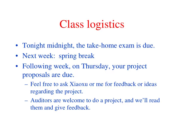
Class logistics

• Tonight midnight, the take-home exam is due.
• Next week: spring break
• Following week, on Thursday, your project

proposals are due.

– Feel free to ask Xiaoxu or me for feedback or ideas regarding the project. – Auditors are welcome to do a project, and we’ll read them and give feedback.

Generative Models

Bill Freeman, MIT

Some of these slides made with Andrew Blake, Microsoft Research Cambridge, UK

6.869 March 17, 2005

Last class

(a) We looked at ways to fit observations of probabilistic data, and EM. (b) We’re looking at the modularized joint probability distribution described by graphical models.

Making probability distributions modular, and therefore tractable:

Probabilistic graphical models

Vision is a problem involving the interactions of many variables: things can seem hopelessly complex. Everything is made tractable, or at least, simpler, if we modularize the problem. That’s what probabilistic graphical models do, and let’s examine that. Readings: Jordan and Weiss intro article—fantastic! Kevin Murphy web page—comprehensive and with pointers to many advanced topics

A toy example

Suppose we have a system of 5 interacting variables, perhaps some are

• bserved and some are not. There’s some probabilistic relationship between

the 5 variables, described by their joint probability, P(x1, x2, x3, x4, x5). If we want to find out what the likely state of variable x1 is (say, the position of the hand of some person we are observing), what can we do? Two reasonable choices are: (a) find the value of x1 (and of all the other variables) that gives the maximum of P(x1, x2, x3, x4, x5); that’s the MAP solution. Or (b) marginalize over all the other variables and then take the mean or the maximum of the other variables. Marginalizing, then taking the mean, is equivalent to finding the MMSE solution. Marginalizing, then taking the max, is called the max marginal solution and sometimes a useful thing to do.

To find the marginal probability at x1, we have to take this sum:

) , , , , (

5 4 3 2

, , , 5 4 3 2 1

∑

x x x x

x x x x x P

If the system really is high dimensional, that will quickly become

• intractable. But if there is some modularity in

then things become tractable again.

) , , , , (

5 4 3 2 1

x x x x x P

Suppose the variables form a Markov chain: x1 causes x2 which causes x3,

• etc. We might draw out this relationship as follows:

1

x

2

x

3

x

4

x

5

x

P(a,b) = P(b|a) P(a) By the chain rule, for any probability distribution, we have: ) | , , , ( ) ( ) , , , , (

1 5 4 3 2 1 5 4 3 2 1

x x x x x P x P x x x x x P =

) , | , , ( ) | ( ) (

2 1 5 4 3 1 2 1

x x x x x P x x P x P = ) , , | , ( ) , | ( ) | ( ) (

3 2 1 5 4 2 1 3 1 2 1

x x x x x P x x x P x x P x P = ) , , , | ( ) , , | ( ) , | ( ) | ( ) (

4 3 2 1 5 3 2 1 4 2 1 3 1 2 1

x x x x x P x x x x P x x x P x x P x P = ) | ( ) | ( ) | ( ) | ( ) (

4 5 3 4 2 3 1 2 1

x x P x x P x x P x x P x P =

But if we exploit the assumed modularity of the probability distribution over the 5 variables (in this case, the assumed Markov chain structure), then that expression simplifies:

1

x

2

x

3

x

4

x

5

x

Now our marginalization summations distribute through those terms:

∑ ∑ ∑ ∑ ∑ ∑

=

1 2 3 4 5 5 4 3 2

) | ( ) | ( ) | ( ) | ( ) ( ) , , , , (

4 5 3 4 2 3 1 2 1 , , , 5 4 3 2 1 x x x x x x x x x

x x P x x P x x P x x P x P x x x x x P

Belief propagation

Performing the marginalization by doing the partial sums is called “belief propagation”.

∑ ∑ ∑ ∑ ∑ ∑

=

1 2 3 4 5 5 4 3 2

) | ( ) | ( ) | ( ) | ( ) ( ) , , , , (

4 5 3 4 2 3 1 2 1 , , , 5 4 3 2 1 x x x x x x x x x

x x P x x P x x P x x P x P x x x x x P

In this example, it has saved us a lot of computation. Suppose each variable has 10 discrete states. Then, not knowing the special structure

• f P, we would have to perform 10000 additions (10^4) to marginalize
• ver the four variables.

But doing the partial sums on the right hand side, we only need 40 additions (10*4) to perform the same marginalization!

1

x

2

x

3

x

4

x

5

x

Another modular probabilistic structure, more common in vision problems, is an undirected graph: The joint probability for this graph is given by:

) , ( ) , ( ) , ( ) , ( ) , , , , (

5 4 4 3 3 2 2 1 5 4 3 2 1

x x x x x x x x x x x x x P Φ Φ Φ Φ =

Where is called a “compatibility function”. We can define compatibility functions we result in the same joint probability as for the directed graph described in the previous slides; for that example, we could use either form.

) , (

2 1 x

x Φ

Markov Random Fields

• Allows rich probabilistic models for

images.

• But built in a local, modular way. Learn

local relationships, get global effects out.

MRF nodes as pixels

Winkler, 1995, p. 32

MRF nodes as patches

image patches Φ(xi, yi) Ψ(xi, xj)

image scene

scene patches

Network joint probability

scene Scene-scene compatibility function neighboring scene nodes image local

• bservations

Image-scene compatibility function

∏ ∏

Φ Ψ =

i i i j i j i

y x x x Z y x P ) , ( ) , ( 1 ) , (

,

In order to use MRFs:

• Given observations y, and the parameters of

the MRF, how infer the hidden variables, x?

• How learn the parameters of the MRF?

Outline of MRF section

• Inference in MRF’s.

– Gibbs sampling, simulated annealing – Iterated condtional modes (ICM) – Variational methods – Belief propagation – Graph cuts

• Vision applications of inference in MRF’s.
• Learning MRF parameters.

– Iterative proportional fitting (IPF)

Variational methods

• Reference: Tommi Jaakkola’s tutorial on

variational methods, http://www.ai.mit.edu/people/tommi/

• Example: mean field

– For each node

• Calculate the expected value of the node,

conditioned on the mean values of the neighbors.

Outline of MRF section

• Inference in MRF’s.

– Gibbs sampling, simulated annealing – Iterated condtional modes (ICM) – Variational methods – Belief propagation – Graph cuts

• Vision applications of inference in MRF’s.
• Learning MRF parameters.

– Iterative proportional fitting (IPF)

Derivation of belief propagation

y1

) , (

1 1 y

x Φ ) , (

2 1 x

x Ψ ) , (

2 2 y

x Φ ) , (

3 2 x

x Ψ ) , (

3 3 y

x Φ

x1 y2 x2 y3 x3

) , , , , , ( sum sum mean

3 2 1 3 2 1 1

3 2 1

y y y x x x P x

x x x MMSE =

The posterior factorizes

) , ( ) , ( sum ) , ( ) , ( sum ) , ( mean ) , ( ) , ( ) , ( ) , ( ) , ( sum sum mean ) , , , , , ( sum sum mean

3 2 3 3 2 1 2 2 1 1 1 3 2 3 3 2 1 2 2 1 1 1 3 2 1 3 2 1 1

3 2 1 3 2 1 3 2 1

x x y x x x y x y x x x x y x x x y x y x x y y y x x x P x

x x x MMSE x x x MMSE x x x MMSE

Ψ Φ Ψ Φ Φ = Ψ Φ Ψ Φ Φ = =

y1

) , (

x Φ ) , (

x Ψ ) , (

x Φ ) , (

x Ψ ) , (

x Φ

x1 y2 x2 y3 x3

Propagation rules

y1

) , (

x Φ ) , (

x Ψ ) , (

x Φ ) , (

x Ψ ) , (

x Φ

x1 y2 x2 y3 x3

) , ( ) , ( sum ) , ( ) , ( sum ) , ( mean ) , ( ) , ( ) , ( ) , ( ) , ( sum sum mean ) , , , , , ( sum sum mean

3 2 3 3 2 1 2 2 1 1 1 3 2 3 3 2 1 2 2 1 1 1 3 2 1 3 2 1 1

3 2 1 3 2 1 3 2 1

x x y x x x y x y x x x x y x x x y x y x x y y y x x x P x

x x x MMSE x x x MMSE x x x MMSE

Ψ Φ Ψ Φ Φ = Ψ Φ Ψ Φ Φ = =

Propagation rules

y1

) , (

x Φ ) , (

x Ψ ) , (

x Φ ) , (

x Ψ ) , (

x Φ

x1 y2 x2 y3 x3

) , ( ) , ( sum ) , ( ) , ( sum ) , ( mean

3 2 3 3 2 1 2 2 1 1 1

3 2 1

x x y x x x y x y x x

x x x MMSE

Ψ Φ Ψ Φ Φ = ) ( ) , ( ) , ( sum ) (

2 3 2 2 2 2 1 1 2 1

2

x M y x x x x M

x

Φ Ψ =

Propagation rules

y1

) , (

x Φ ) , (

x Ψ ) , (

x Φ ) , (

x Ψ ) , (

x Φ

x1 y2 x2 y3 x3

) , ( ) , ( sum ) , ( ) , ( sum ) , ( mean

3 2 3 3 2 1 2 2 1 1 1

3 2 1

x x y x x x y x y x x

x x x MMSE

Ψ Φ Ψ Φ Φ = ) ( ) , ( ) , ( sum ) (

2 3 2 2 2 2 1 1 2 1

2

x M y x x x x M

x

Φ Ψ =

Belief propagation: the nosey neighbor rule

“Given everything that I know, here’s what I think you should think” (Given the probabilities of my being in different states, and how my states relate to your states, here’s what I think the probabilities of your states should be)

Belief propagation messages

A message: can be thought of as a set of weights on each of your possible states To send a message: Multiply together all the incoming messages, except from the node you’re sending to, then multiply by the compatibility matrix and marginalize

• ver the sender’s states.

∏ ∑

∈

=

i j N k j k j j i x i j i

x M x x x M

j

\ ) ( ij

) ( ) , ( ) ( ψ

j i

=

j i

Beliefs

To find a node’s beliefs: Multiply together all the messages coming in to that node. j

∏

∈

=

) (

) ( ) (

j N k j k j j j

x M x b

Belief, and message updates

∏

∈

=

) (

) ( ) (

j N k j k j j j

x M x b

j

∏ ∑

∈

=

i j N k j k j j i x i j i

x M x x x M

j

\ ) ( ij

) ( ) , ( ) ( ψ

=

j i i

Optimal solution in a chain or tree: Belief Propagation

• “Do the right thing” Bayesian algorithm.
• For Gaussian random variables over time:

Kalman filter.

• For hidden Markov models:

forward/backward algorithm (and MAP variant is Viterbi).

No factorization with loops!

y1 x1 y2 x2 y3 x3

) , ( ) , ( sum ) , ( ) , ( sum ) , ( mean

3 2 3 3 2 1 2 2 1 1 1

3 2 1

x x y x x x y x y x x

x x x MMSE

Ψ Φ Ψ Φ Φ =

3 1

) , ( x x Ψ

Justification for running belief propagation in networks with loops

• Experimental results:

– Error-correcting codes – Vision applications

• Theoretical results:

– For Gaussian processes, means are correct. – Large neighborhood local maximum for MAP. – Equivalent to Bethe approx. in statistical physics. – Tree-weighted reparameterization Weiss and Freeman, 2000 Yedidia, Freeman, and Weiss, 2000 Freeman and Pasztor, 1999; Frey, 2000 Kschischang and Frey, 1998; McEliece et al., 1998 Weiss and Freeman, 1999 Wainwright, Willsky, Jaakkola, 2001

Statistical mechanics interpretation

U - TS = Free energy U = avg. energy = T = temperature S = entropy =

,...) , ( ,...) , (

2 1 2 1

x x E x x p

states

∑

,...) , ( ln ,...) , (

2 1 2 1

x x p x x p

states

∑

−

Free energy formulation

Defining then the probability distribution that minimizes the F.E. is precisely the true probability of the Markov network,

) ( ) , ( ,...) , (

2 1 i i i j i ij ij

x x x x x P

∏ ∏

Φ Ψ =

,...) , (

2 1 x

x P

T x x E j i ij

j i

e x x

/ ) , (

) , (

−

= Ψ

T x E i i

i

e x

/ ) (

) (

−

= Φ

Approximating the Free Energy

Exact: Mean Field Theory: Bethe Approximation : Kikuchi Approximations:

)] ,..., , ( [

2 1 N

x x x p F

)] ( [

i i x

b F

)] , ( ), ( [

j i ij i i

x x b x b F

),....] , ( ), , ( ), ( [

, k j i ijk j i ij i i

x x x b x x b x b F

Mean field approximation to free energy

U - TS = Free energy

∑∑ ∑∑

+ =

) ( ,

) ( ln ) ( ) , ( ) ( ) ( ) (

ij x x i i i i i x j i ij j j i i i MeanField

j i i

x b T x b x x E x b x b b F

The variational free energy is, up to an additive constant, equal to the Kllback-Leibler divergence between b(x) and the true probability, P(x). KL divergence:

) ( ) ( ln ) ( ) || (

,... , 2

1

x P x b x b P b D

i i i i x x KL

∏ ∏ ∑

=

Setting deriv w.r.t bi=0

U - TS = Free energy

Corresponds to eq. 18 in Jordan and Weiss ms.

∑∑

− =

) (

) / ) , ( ) ( exp( ) (

ij x j i ij j j i i

j

T x x E x b x b α

In words: “Set the probability of each state xi at node i to be proportional to e to the minus expected energy corresponding to each state xi, given the expected values of all the neighboring states.”

Bethe Approximation

On tree-like lattices, exact formula:

∏ ∏

−

=

i q i i ij j i ij N

i

x p x x p x x x p

1 ) ( 2 1

)] ( [ ) , ( ) ,..., , (

∑∑

+ =

) ( ,

)) , ( ln ) , ( )( , ( ) , (

ij x x j i ij j i ij j i ij ij i Bethe

j i

x x b T x x E x x b b b F

∑ ∑

+ − +

i x i i i i i i i

i

x b T x E x b q )) ( ln ) ( )( ( ) 1 (

Gibbs Free Energy

)} ( ) , ( ){ ( } 1 ) , ( { ) , (

) ( , ) ( j j x j i ij j ij ij x x x j i ij ij ij ij i Bethe

x b x x b x x x b b b F

i j j i

− + − +

∑ ∑ ∑ ∑ ∑

λ γ

Gibbs Free Energy

)} ( ) , ( ){ ( } 1 ) , ( { ) , (

) ( , ) ( j j x j i ij j ij ij x x x j i ij ij ij ij i Bethe

x b x x b x x x b b b F

i j j i

− + − +

∑ ∑ ∑ ∑ ∑

λ γ

Set derivative of Gibbs Free Energy w.r.t. bij, bi terms to zero:

) exp( ) ( ) ( ) ) ( exp( ) , ( ) , (

) ( ) (

T x k x b T x x x k x x b

i N j i x ij i i i i ij j i ij j i ij ∑ ∈

Φ = − Ψ =

λ

λ

Belief Propagation = Bethe

∑

=

i

x j i ij j j

x x b x b ) , ( ) (

) (

j ij x

λ

Lagrange multipliers enforce the constraints

Bethe stationary conditions = message update rules

∏

∈

=

i j N k j k j j ij

x M T x

\ ) (

) ( ln ) ( λ

with

Region marginal probabilities

) ( ) ( ) , ( ) , ( ) ( ) ( ) (

\ ) ( \ ) ( ) (

∏ ∏ ∏

∈ ∈ ∈

Ψ = Φ =

i j N k j k j j i N k i k i j i j i ij i N k i k i i i i

x M x M x x k x x b x M x k x b

i j i

Belief propagation equations

Belief propagation equations come from the marginalization constraints.

j i i j

=

i i

∏ ∑

∈

=

i j N k j k j j i x i j i

x M x x x M

j

\ ) ( ij

) ( ) , ( ) ( ψ

Results from Bethe free energy analysis

• Fixed point of belief propagation equations iff. Bethe

approximation stationary point.

• Belief propagation always has a fixed point.
• Connection with variational methods for inference: both

minimize approximations to Free Energy,

– variational: usually use primal variables. – belief propagation: fixed pt. equs. for dual variables.

• Kikuchi approximations lead to more accurate belief

propagation algorithms.

• Other Bethe free energy minimization algorithms—

Yuille, Welling, etc.

Kikuchi message-update rules

Groups of nodes send messages to other groups of nodes.

Typical choice for Kikuchi cluster.

i j i j

=

i j i

=

l k

Update for messages Update for messages

Generalized belief propagation

Marginal probabilities for nodes in one row

• f a 10x10 spin glass

References on BP and GBP

• J. Pearl, 1985

– classic

• Y. Weiss, NIPS 1998

– Inspires application of BP to vision

• W. Freeman et al learning low-level vision, IJCV 1999

– Applications in super-resolution, motion, shading/paint discrimination

• H. Shum et al, ECCV 2002

– Application to stereo

• M. Wainwright, T. Jaakkola, A. Willsky

– Reparameterization version

• J. Yedidia, AAAI 2000

– The clearest place to read about BP and GBP.

Graph cuts

• Algorithm: uses node label swaps or expansions

as moves in the algorithm to reduce the energy. Swaps many labels at once, not just one at a time, as with ICM.

• Find which pixel labels to swap using min cut/max

flow algorithms from network theory.

• Can offer bounds on optimality.
• See Boykov, Veksler, Zabih, IEEE PAMI 23 (11)
• Nov. 2001 (available on web).

Comparison of graph cuts and belief propagation

Comparison of Graph Cuts with Belief Propagation for Stereo, using Identical MRF Parameters, ICCV 2003. Marshall F. Tappen William T. Freeman

Ground truth, graph cuts, and belief propagation disparity solution energies

Graph cuts versus belief propagation

• Graph cuts consistently gave slightly lower energy

solutions for that stereo-problem MRF, although BP ran faster, although there is now a faster graph cuts implementation than what we used…

• However, here’s why I still use Belief

Propagation:

– Works for any compatibility functions, not a restricted set like graph cuts. – I find it very intuitive. – Extensions: sum-product algorithm computes MMSE, and Generalized Belief Propagation gives you very accurate solutions, at a cost of time.

MAP versus MMSE

Show program comparing some methods on a simple MRF

testMRF.m

Outline of MRF section

• Inference in MRF’s.

– Gibbs sampling, simulated annealing – Iterated condtional modes (ICM) – Variational methods – Belief propagation – Graph cuts

• Vision applications of inference in MRF’s.
• Learning MRF parameters.

– Iterative proportional fitting (IPF)

Vision applications of MRF’s

• Stereo
• Motion estimation
• Super-resolution
• Many others…

Vision applications of MRF’s

• Stereo
• Motion estimation
• Super-resolution
• Many others…

Motion application

image patches

image scene

scene patches

What behavior should we see in a motion algorithm?

• Aperture problem
• Resolution through propagation of

information

• Figure/ground discrimination

The aperture problem

The aperture problem

Program demo

Motion analysis: related work

• Markov network

– Luettgen, Karl, Willsky and collaborators.

• Neural network or learning-based

– Nowlan & T. J. Senjowski; Sereno.

• Optical flow analysis

– Weiss & Adelson; Darrell & Pentland; Ju, Black & Jepson; Simoncelli; Grzywacz & Yuille; Hildreth; Horn & Schunk; etc.

Motion estimation results

(maxima of scene probability distributions displayed)

Inference:

Image data Initial guesses only show motion at edges. Iterations 0 and 1

Motion estimation results

(maxima of scene probability distributions displayed)

Figure/ground still unresolved here. Iterations 2 and 3

Motion estimation results

(maxima of scene probability distributions displayed)

Iterations 4 and 5 Final result compares well with vector quantized true (uniform) velocities.

Vision applications of MRF’s

• Stereo
• Motion estimation
• Super-resolution
• Many others…

Super-resolution

• Image: low resolution image
• Scene: high resolution image

ultimate goal...

image scene

Polygon-based graphics images are resolution independent Pixel-based images are not resolution independent Pixel replication Cubic spline Cubic spline, sharpened Training-based super-resolution

3 approaches to perceptual sharpening

(1) Sharpening; boost existing high frequencies. (2) Use multiple frames to obtain higher sampling rate in a still frame. (3) Estimate high frequencies not present in image, although implicitly defined.

In this talk, we focus on (3), which we’ll call “super-resolution”.

spatial frequency amplitude spatial frequency amplitude

Super-resolution: other approaches

• Schultz and Stevenson, 1994
• Pentland and Horowitz, 1993
• fractal image compression (Polvere, 1998;

Iterated Systems)

• astronomical image processing (eg. Gull and

Daniell, 1978; “pixons” http://casswww.ucsd.edu/puetter.html)

Training images, ~100,000 image/scene patch pairs

Images from two Corel database categories: “giraffes” and “urban skyline”.

Do a first interpolation

Zoomed low-resolution Low-resolution

Zoomed low-resolution Full frequency original Low-resolution

Representation

Zoomed low-freq. Full freq. original

Representation

Zoomed low-freq. Full freq. original True high freqs

(to minimize the complexity of the relationships we have to learn, we remove the lowest frequencies from the input image, and normalize the local contrast level).

Low-band input (contrast normalized, PCA fitted)

Gather ~100,000 patches

...

Training data samples (magnified)

...

high freqs. low freqs.

True high freqs. Input low freqs. Training data samples (magnified)

...

Nearest neighbor estimate

...

high freqs. Estimated high freqs. low freqs.

Input low freqs. Training data samples (magnified)

...

Nearest neighbor estimate

Estimated high freqs.

...

high freqs. low freqs.

Example: input image patch, and closest matches from database

Input patch Closest image patches from database Corresponding high-resolution patches from database

Scene-scene compatibility function, Ψ(xi, xj)

Assume overlapped regions, d, of hi-res. patches differ by Gaussian observation noise:

d

Uniqueness constraint, not smoothness.

y

Image-scene compatibility function, Φ(xi, yi)

x

Assume Gaussian noise takes you from

• bserved image patch to synthetic sample:

Markov network

image patches Φ(xi, yi) Ψ(xi, xj) scene patches

Belief Propagation

Input

• Iter. 0

After a few iterations of belief propagation, the algorithm selects spatially consistent high resolution interpretations for each low-resolution patch of the input image.

• Iter. 1
• Iter. 3

Zooming 2 octaves

We apply the super-resolution algorithm recursively, zooming up 2 powers of 2, or a factor of 4 in each dimension. 85 x 51 input Cubic spline zoom to 340x204

• Max. likelihood zoom to 340x204

Now we examine the effect of the prior assumptions made about images on the high resolution reconstruction. First, cubic spline interpolation.

Original 50x58 (cubic spline implies thin plate prior) True 200x232

Original 50x58 (cubic spline implies thin plate prior) True 200x232 Cubic spline

Next, train the Markov network algorithm on a world of random noise images.

Original 50x58 Training images True

The algorithm learns that, in such a world, we add random noise when zoom to a higher resolution.

Original 50x58 Training images Markov network True

Next, train on a world of vertically

• riented rectangles.

Original 50x58 Training images True

The Markov network algorithm hallucinates those vertical rectangles that it was trained on.

Original 50x58 Training images Markov network True

Training images

Now train on a generic collection of images.

Original 50x58 True

The algorithm makes a reasonable guess at the high resolution image, based on its training images.

Training images Original 50x58 Markov network True

Generic training images

Next, train on a generic set of training images. Using the same camera as for the test image, but a random collection of photographs.

Original 70x70 Cubic Spline Markov net, training: generic True 280x280

Kodak Imaging Science Technology Lab test.

3 test images, 640x480, to be zoomed up by 4 in each dimension. 8 judges, making 2-alternative, forced-choice comparisons.

Algorithms compared

• Bicubic Interpolation
• Mitra's Directional Filter
• Fuzzy Logic Filter
• Vector Quantization
• VISTA

Bicubic spline Altamira VISTA

Bicubic spline Altamira VISTA

User preference test results

“The observer data indicates that six of the observers ranked Freeman’s algorithm as the most preferred of the five tested

• algorithms. However the other two observers rank Freeman’s algorithm

as the least preferred of all the algorithms…. Freeman’s algorithm produces prints which are by far the sharpest

• ut of the five algorithms. However, this sharpness comes at a price
• f artifacts (spurious detail that is not present in the original

scene). Apparently the two observers who did not prefer Freeman’s algorithm had strong objections to the artifacts. The other observers apparently placed high priority on the high level of sharpness in the images created by Freeman’s algorithm.”

Training images

Training image

Processed image

Outline of MRF section

• Inference in MRF’s.

– Gibbs sampling, simulated annealing – Iterated conditional modes (ICM) – Variational methods – Belief propagation – Graph cuts

• Vision applications of inference in MRF’s.
• Learning MRF parameters.

– Iterative proportional fitting (IPF)

Learning MRF parameters, labeled data

Iterative proportional fitting lets you make a maximum likelihood estimate of a joint distribution from

• bservations of various marginal

distributions.

True joint probability Observed marginal distributions

Initial guess at joint probability

IPF update equation

Scale the previous iteration’s estimate for the joint probability by the ratio of the true to the predicted marginals. Gives gradient ascent in the likelihood of the joint probability, given the observations of the marginals.

See: Michael Jordan’s book on graphical models

Convergence of to correct marginals by IPF algorithm

Convergence of to correct marginals by IPF algorithm

IPF results for this example: comparison of joint probabilities

True joint probability Initial guess Final maximum entropy estimate

Application to MRF parameter estimation

• Can show that for the ML estimate of the clique

potentials, φc(xc), the empirical marginals equal the model marginals,

• This leads to the IPF update rule for φc(xc)
• Performs coordinate ascent in the likelihood of the

MRF parameters, given the observed data.

Reference: unpublished notes by Michael Jordan

More general graphical models than MRF grids

• In this course, we’ve studied Markov chains, and

Markov random fields, but, of course, many other structures of probabilistic models are possible and useful in computer vision.

• For a nice on-line tutorial about Bayes nets, see

Kevin Murphy’s tutorial in his web page.

“Top-down” information: a representation for image context

Images 80-dimensional representation

Credit: Antonio Torralba

“Bottom-up” information: labeled training data for object recognition.

• Hand-annotated 1200 frames of video from a wearable webcam
• Trained detectors for 9 types of objects: bookshelf, desk,

screen (frontal) , steps, building facade, etc.

• 100-200 positive patches, > 10,000 negative patches

Combining top-down with bottom-up: graphical model showing assumed statistical relationships between variables

Scene category Visual “gist”

• bservations

Object class Particular objects Local image features

kitchen, office, lab, conference room, open area, corridor, elevator and street.

Categorization of new places

ICCV 2003 poster By Torralba, Murphy, Freeman, and Rubin

Specific location Location category Indoor/outdoor

frame

Bottom-up detection: ROC curves

ICCV 2003 poster By Torralba, Murphy, Freeman, and Rubin