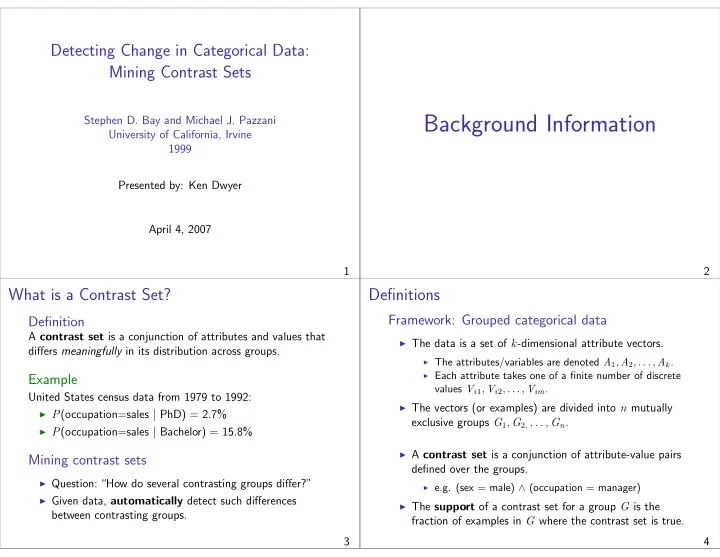

Detecting Change in Categorical Data: Mining Contrast Sets Background Information Stephen D. Bay and Michael J. Pazzani University of California, Irvine 1999 Presented by: Ken Dwyer April 4, 2007 1 2 What is a Contrast Set? Definitions Framework: Grouped categorical data Definition A contrast set is a conjunction of attributes and values that ◮ The data is a set of k -dimensional attribute vectors. differs meaningfully in its distribution across groups. ◮ The attributes/variables are denoted A 1 , A 2 , . . . , A k . ◮ Each attribute takes one of a finite number of discrete Example values V i 1 , V i 2 , . . . , V im . United States census data from 1979 to 1992: ◮ The vectors (or examples) are divided into n mutually ◮ P (occupation=sales | PhD) = 2.7% exclusive groups G 1 , G 2 , . . . , G n . ◮ P (occupation=sales | Bachelor) = 15.8% ◮ A contrast set is a conjunction of attribute-value pairs Mining contrast sets defined over the groups. ◮ Question: “How do several contrasting groups differ?” ◮ e.g. (sex = male) ∧ (occupation = manager) ◮ Given data, automatically detect such differences ◮ The support of a contrast set for a group G is the between contrasting groups. fraction of examples in G where the contrast set is true. 3 4
Mining Contrast Sets: Objective Formally, find contrast sets ‘cset’ where: Background Information 1. ∃ ij P (cset = True | G i ) � = P (cset = True | G j ) 2. max ij | support(cset, G i ) − support(cset, G j ) | ≥ δ ◮ δ is a threshold called the minimum support difference Na ¨ ı ve Approach Definitions A contrast set is . . . ◮ significant if Equation 1 is statistically valid. ◮ large if Equation 2 is satisfied. ◮ a deviation if both requirements are met. 5 6 Na ¨ ı ve Approach Na ¨ ı ve Approach Association Rule Learning with a Group Variable Shortcomings Problem definition re-visited Find conjunctions of attributes and values that have different ◮ The number of rules discovered is large: levels of support in different groups. ◮ For US census data: 26,796 rules for Bachelor group, 1,674 for PhD group (1% min supp, 80% min conf). Apply association rule learning! ◮ Main problem: The association rule learner does not enforce consistent contrast [DB96]: ◮ Association rule learners [AS94] can discover relationships ◮ The same attributes are not necessarily used to compare between attributes in a dataset. the groups. ◮ Idea: Add a group attribute to the data and run the ◮ At least 25,122 of the PhD rules have no match. association rule learner to find group differences. ◮ Are the differences in support and confidence statistically significant? 7 8
STUCCO: An Algorithm for Mining Contrast Sets Search and Testing for Understandable Consistent COntrasts ◮ Construct a search tree in which the root node is the Background Information empty contrast set. ◮ Generate a node’s children by adding a new attribute-value pair, based on an ordering of such pairs. ◮ Search in a breadth-first manner, counting the support Na ¨ ı ve Approach for each group in a level as we proceed. The STUCCO Algorithm 9 10 Finding Significant Contrast Sets Finding Significant Contrast Sets Chi-square test for independence Statistical hypothesis testing ◮ χ 2 = � r ( o ij − e ij ) 2 � c i = 1 j = 1 e ij ◮ Null hypothesis: Contrast set support is equal across all groups (support is independent of group membership). Arts Bio. Eng. ICS SocEc Total SATV > 700 45 142 85 60 11 343 ◮ Form a 2 × | G | contingency table. ¬ (SATV > 700) 583 2465 1523 502 414 5487 Total 628 2607 1608 562 425 5830 Example ◮ Consider cell 1,1: e 1 , 1 = ( 343 · 628 ) / 5830 = 36 . 95 SAT Verbal scores for different UCI schools: ◮ Cell contributes ( 45 − 36 . 95 ) 2 / 36 . 95 = 1 . 75 to χ 2 ◮ In total, we get χ 2 = 35 . 4 Arts Bio. Eng. ICS SocEc SATV > 700 45 142 85 60 11 1. Choose a significance level α ¬ (SATV > 700) 583 2465 1523 502 414 2. Calculate the p-value p High scores (%) 7.2 5.4 5.3 10.7 2.6 3. Reject the null hypothesis if p < α ◮ In this case, we compute p = 3 . 8 e − 7 ◮ For α = . 05 , ‘SATV > 700’ is significant. 11 12
Controlling Type I Error Pruning ◮ Idea: If none of the children (specializations) of a node Type I error (false positive) can possibly be significant and large, then the node is ◮ Occurs when the null hypothesis is falsely rejected. pruned from the search tree. ◮ The maximum probability of such an error is α . ◮ e.g. With 1000 tests at α = .05, we could detect 50 Pruning criteria significant differences, even if there really are none. 1. Minimum deviation size Bonferroni method (see [Sha95]) 2. Expected cell frequencies 3. Chi-square bounds ◮ Choose a significance level α i for the i th test such that � i α i ≤ α (1) Recall: The maximum difference between the support of ◮ Traditionally, for n tests, α i = α/ n any two groups must be at least δ for the contrast set to be large. This is not possible for the children of a node unless at ◮ STUCCO: For level l , use α l = min ( 2 l ·| C l | , α l − 1 ) α least one group’s support is greater than δ . ◮ | C l | is the number of candidates at level l . 13 14 Pruning Pruning ◮ Idea: If none of the children (specializations) of a node ◮ Idea: If none of the children (specializations) of a node can possibly be significant and large, then the node is can possibly be significant and large, then the node is pruned from the search tree. pruned from the search tree. Pruning criteria Pruning criteria 1. Minimum deviation size 1. Minimum deviation size 2. Expected cell frequencies 2. Expected cell frequencies 3. Chi-square bounds 3. Chi-square bounds (3) An upper bound on the χ 2 statistic can be be computed for (2) The expected cell frequencies in the top row of the con- tingency table cannot possibly increase as new attributes are any child node. A candidate is pruned if further specializations The χ 2 test is invalid for small added to the contrast set. cannot possibly meet the α l significance cutoff. counts (i.e. < 5), and so the node is pruned in such cases. 14 14
Surprising Contrast Sets ◮ Idea: Only show those contrast sets that are surprising Background Information given what has already been shown. Example Na ¨ ı ve Approach ◮ Suppose we know the following: ◮ P (sex=male | PhD) = .81 ◮ P (occupation=manager | PhD) = .14 The STUCCO Algorithm ◮ Assuming independence, we expect that: ◮ P (male ∧ manager | PhD) = .81 × .14 = .113 Experimental Evaluation ◮ The actual probability is .109, which is not surprising in this sense. ◮ Iterative proportional fitting [Eve92] is used to find the MLEs for a conjunction of variables based on its subsets. 15 16 Experimental Evaluation Experimental Evaluation Results for US Census data ◮ Two datasets; continuous attributes discretized. Observed % Expected % χ 2 Contrast Set PhD Bach. PhD Bach. p workclass = State-gov 21.0 5.4 225.1 6.9e-51 1. US Census [NHBM98] – 48,842 examples; 14 attributes. occupation = sales 2.7 15.8 74.9 4.8e-18 hour per week > 60 8.4 3.2 43.4 4.4e-11 ◮ “What are the differences between people with PhD and native country = U.S. 80.5 89.5 45.9 1.3e-11 Bachelor degrees?” ( δ = 1%, α = .05) native country = Canada 1.9 0.5 18.6 1.6e-5 native country = India 1.6 0.5 15.2 9.5e-5 2. UCI Admissions – 6 years of data with ∼ 17,000 examples salary > 50K 72.6 41.3 220.2 8.3e-50 sex = male 61.8 34.8 58.8 28.5 173.6 1.2e-39 per year; 17 attributes. ∧ salary > 50K occupation = prof-specialty 7.6 2.6 10.7 3.5 48.2 3.8e-12 ◮ “How has the applicant pool changed from 1993-1998?” ∧ sex = female ( δ = 5%, α = .05) ∧ salary > 50K 17 18
Experimental Evaluation Experimental Evaluation Results for UCI Admissions data Effectiveness of Pruning ‘Admit = Yes ∧ SAT Verbal < 400’ ◮ Graph plots number of candidates counted at each level. ◮ Deviation size pruning (dashed) versus all three pruning methods (solid). ◮ Census (left) and UCI Admissions in 1998 (right). (Expected values are indicated by the dotted lines) 19 20 Concluding Remarks Background Information Summary ◮ Motivated the problem of identifying differences between Na ¨ ı ve Approach several groups. ◮ Defined a contrast set, and proposed the STUCCO algorithm for mining meaningful contrast sets. The STUCCO Algorithm ◮ Demonstrated STUCCO’s utility on two real datasets. Experimental Evaluation Key Strengths ◮ Formulated a statistically grounded approach. Concluding Remarks ◮ Introduced pruning strategies that are specific to contrast set mining. ◮ Concentrated on keeping the results compact. 21 22
Selected References R. Agrawal and R. Srikant. Fast algorithms for mining association rules in large databases. In Proc. 20th International Conference on Very Large Data Bases , pages 487–499, 1994. S.D. Bay and M.J. Pazzani. Detecting change in categorical data: mining contrast sets. Proc. 5th ACM SIGKDD International Conference on Knowledge Discovery and Data Mining , pages 302–306, 1999. J. Davies and D. Billman. Hierarchical categorization and the effects of contrast inconsistency in an unsupervised learning task. In Proc. 18th Annual Conference of the Cognitive Science Society , page 750, 1996. B.S. Everitt. The analysis of contingency tables . Chapman and Hall, second edition, 1992. D. J. Newman, S. Hettich, C. L. Blake, and C. J. Merz. UCI repository of machine learning databases, 1998. J.P. Shaffer. Multiple hypothesis testing. Annual Review of Psychology , 46:561–584, 1995. 23
Recommend
More recommend