Child-Related Transfers, Household Labor Supply and Welfare Nezih - PowerPoint PPT Presentation
Child-Related Transfers, Household Labor Supply and Welfare Nezih Guner, Remzi Kaygusuz and Gustavo Ventura CEMFI Tilburg University Arizona State University January 2017 Motivation Availability and cost of childcare is a key determinant
Child-Related Transfers, Household Labor Supply and Welfare Nezih Guner, Remzi Kaygusuz and Gustavo Ventura CEMFI Tilburg University Arizona State University January 2017
Motivation � Availability and cost of childcare is a key determinant of female labor supply. � The macroeconomic and welfare implications of Child-Related Transfers to households. � Childcare subsidies � Child-related tax credits � What are the labor supply, gender gap, output, and welfare e¤ects for the US economy?
What we do � Develop a life-cycle economy with heterogenous married and single agents, household labor supply decisions and costly childbearing – Guner, Kaygusuz and Ventura (2012). � Parameterize this model to be consistent with a host of cross-sectional observations. � gender and skill premia, labor force participation of married females, structure of marital sorting, and the cost of children. � Use framework for a quantitative evaluation of Child-Related Transfers.
Why We Care � Female labor supply is quite elastic. Potentially large e¤ects. � Big interest in policy circles: Child-related transfers are appealing form of government transfers – without negative e¤ects on labor supply. � Such transfers are substantial in some countries (e.g Sweden), but rather small in the U.S. � President Obama’s 2015 State of the Union Address: � "In today’s economy, when having both parents in the workforce is an economic necessity for many families, we need a¤ordable, high-quality childcare more than ever. It is not a nice-to-have — it is a must–have. So it is time we stop childcare as a side issue, or a women’s issue, and treat it like a national economic priority that is for all of us.” � Both Clinton and Trump were proposing expansions of child-related transfers.
Child-Related Transfers in the US � Child-Care Subsidies � Means-tested, conditional on work. Serves mainly poor working households. � Approximately 1.71 million children in 201, about 5.5% of children between ages 0 to 13. � Subsidy rate is about 75%. � Child-Tax Credits (CTC) � Means-tested, partly-refundable tax credit. � Independent of childcare expenditures or labor market status of parents. � Starts at 1000$ per child and declines by income. � Child and Dependent Care Tax Credit (CDCTC) � Non-refundable tax credit for child care expenditures for all households with working parents. � Maximum credit is 1050$ per child (with an overall maximum of 2010$), and declines by household income. � Serves middle and high income working households.
Key Model Features � Extensive margin in heterogenous couples. � Permits quanti…cation of major sources of labor-supply gains. � Account for costly childbearing in married and single households. � Permits clean analysis of expansion of current arrangements. � Model skill depreciation of females due to childbearing disruptions. � Allows us to capture increases in female skills due to expansion of subsidies. � Detailed modelling of existing policies. � Link to current policy debate.
Related Literature � Heckman (1974), Hotz and Miller (1988), Blau and Hagy (1998): the e¤ect of childcare costs on female labor supply � Attanasio, Low and Sanchez-Marcos (2008): reduction in child care costs and the rise of female labor supply. � Bick (2016): childcare subsidies have quantitatively signi…cant e¤ects on female labor supply. � Domeij and Klein (2013): optimality of childcare subsidies in life-cycle economies. They compute the welfare-maximizing level of childcare subsidies for German economy. � Rogerson (2007) – use of tax revenue to …nance government transfers of service sector goods that are tied to female work
Heterogeneity � Life-cycle economy, j = 1 , ...., J R , .... J . � Males ( m ) and females ( f ) , heterogenous in their types (education). � Male types, z 2 Z . These types map into productivity pro…les, ̟ m ( z , j ) . � Female types, x 2 X . These types map into initial productivity levels, h 1 = ̟ f ( x , 1 ) , and after age 1, h evolves endogenously. h 0 = exp [ ln h + α x χ ( l ) � δ x ( 1 � χ ( l ))] , j |{z} |{z} dep. growth � Additional permanent heterogeneity (within each type). � Male labor endowments: ̟ m ( z , j ) ε z � Female labor endowments: h ε x .
Household Structure � Agents can be single ( S ) or married ( M ) . � Married agents age, retire, and die together. Stationary demographics. � Individuals value consumption and dislike work. Married households dislike joint work. � Married agents maximize discounted sum of individual utilities.
Children and Child Care Costs � Married households and single females di¤er in terms of the number of children attached to them – k ( x ) , k ( x , z ) � They also di¤er whether they have access to informal care, g 2 f 0 , 1 g . � Three possibilities: without any children, early child bearers, late child bearers, denoted by b = f 0 , 1 , 2 g � Early child bearers have children in ages j = 1 , 2 , 3 while late child bearers have children in ages j = 2 , 3 , 4 .
Children and Child Care Costs � If a female with children works, married or single, then the household has to pay for child care costs. � Independent of hours worked. � Child care costs depend on � the age of the child, s = 1 , 2 , 3 . � whether the household has access to informal care, g 2 f 0 , 1 g � the type (education) of the mother. � Amount of child care required, d ( s , x , g ) k ( x ) or d ( s , x , z , g ) k ( x , z ) . � Total cost wd ( s , x , g ) k ( x ) or wd ( s , x , z , g ) k ( x , z ) .
Child Related Transfers • Child care subsidies • Cost of childcare is wd ( s , x , z , g ) k ( x , z )( 1 − θ ) if I ≤ � I , and wd ( s , x , z , g ) k ( x , z ) otherwise. • Two parameters: subsidy rate ( θ ) and eligibility ( � I ). • Tax Credits • CTC — potential credit that start from a maximum, and then declines by income • CDCTC — potential credit = min {maximum credit, earnings, childcare expenditure}*rate • rate declines by household income • CDCTC is not refundable, and CTC is partially refundable. • Actual credit depends on how much household own in taxes.
Other Taxes and Transfers � Households pay taxes on their total income T M ( I , k ) and T S ( I , k ) � captures federal income tax � There is a (‡at) payroll tax that taxes individual labor incomes, represented by τ p , to fund social-security transfers. � Each household pays an additional ‡at capital income tax for the returns from his/her asset holdings, denoted by τ k .
Other Taxes and Transfers � The Earned Income Tax Credits (EITC), which works as a wage subsidy for households below a certain income level. � Each household below a certain income level also receives a transfer from the government as a function of its marital status and income. � Captures the other aspects of the welfare system in the US, such as the TANF and Food Stamps. � For a household with income level I , number of children k and total child care expenditure D , the total tax credits and transfers are represented by TR S f ( I , D , k ) , TR S m ( I , D , k ) and TR M ( I , D , k ) .
Decisions � Households decide how much to consume and how much to save � Married households decide whether the female member of the household should work � Costs of work: child care expenses � Bene…ts: higher household income, human capital accumulation. � Child-related transfers a¤ect the cost and bene…ts of work for married females.
Extensive Margin � At the start of their lives married households draw a shock, q , which stands for the utility costs of joint market work for married couples. � Residual heterogeneity in labor force participation.
Preferences � Single male m ( c , l ) = log ( c ) � ϕ ( l ) 1 + 1 U S γ . � Single female f ( c , l , k y ) = log ( c ) � ϕ ( l + k y η ) 1 + 1 U S γ , � Married male 1 + 1 � 1 U M γ m ( c , l m , l f , q ) = log ( c ) � ϕ l 2 χ f l f g q , m � Married female γ � 1 f ( c , l f , q , k y ) = log ( c ) � ϕ ( l f + k y η ) 1 + 1 U M 2 χ f l f g q , Note: γ is same for males and females
Decision Problem – Married with Children � Let s M � ( x , z , ε x , ε z , q , b , g ) . � For b = f 1 , 2 g , j 2 f b , b + 1 , b + 2 g , V M ( a , h , s M , j ) = a 0 , l f , l m f [ U M f ( c , l f , q , k y ) + U M m ( c , l m , l f , q )] + β V M ( 0 ) g max subject to 8 a ( 1 + r ( 1 � τ k )) + w ( ̟ m ( z , j ) ε z l m + h ε x l f )( 1 � τ p ) > > > > � T M ( I , k ( x , z )) + TR M ( I , D ( 1 � θ ) , k ( x , z )) > > > > � wd ( j + 1 � b , x , z , g ) k ( x , z )( 1 � θ ) χ ( l f ) if I � b < I c + a 0 = > > > a ( 1 + r ( 1 � τ k )) + w ( ̟ m ( z , j ) ε z l m + h ε x l f )( 1 � τ p ) > > > > � T M ( I , k ( x , z )) + TR M ( I , D , k ( x , z )) > : � wd ( j + 1 � b , x , z , g ) k ( x , z ) χ ( l f ) , otherwise where I = w ̟ m ( z , j ) ε z l m + wh ε x l f + ra and D = wd ( j + 1 � b , x , z , g ) k ( x , z ) .
Recommend
More recommend
Explore More Topics
Stay informed with curated content and fresh updates.

