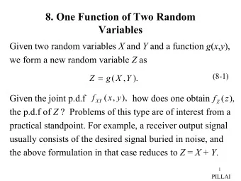
Chapter 4: Multiple Random Variables STK4011/9011: Statistical - PowerPoint PPT Presentation

Chapter 4: Multiple Random Variables STK4011/9011: Statistical Inference Theory Johan Pensar STK4011/9011: Statistical Inference Theory Chapter 4: Multiple Random Variables 1 / 20

Overview Joint and Marginal Distributions 1 Conditional Distributions and Independence 2 Covariance and Correlation 3 Bivariate Transformations 4 Covers Sec 4.1–4.3 and 4.5 in CB. STK4011/9011: Statistical Inference Theory Chapter 4: Multiple Random Variables 2 / 25

Random vectors In most experiments one is interested in more than one random variable. Multivariate probability models: models over multiple random variables (random vector). An n -dimensional random vector X = ( X 1 , . . . , X n ) is a function from a sample space S to R n , that is, X : S → R n . In the following we focus on the bivariate case (two random variables), but the results generalize to the multivariate case with more than two variables. STK4011/9011: Statistical Inference Theory Chapter 4: Multiple Random Variables 3 / 20

Joint Probability Mass Function (PMF) The joint pmf of a discrete random vector ( X , Y ) is defined by f ( x , y ) = P ( X = x , Y = y ) . For any subset (or event) A ⊆ R 2 : X P (( X , Y ) ∈ A ) = f ( x , y ) . ( x , y ) ∈ A Properties of the joint pmf: f ( x , y ) ≥ 0 for all ( x , y ) ∈ R 2 (and f ( x , y ) > 0 for a countable number of outcomes), P ( x , y ) ∈ R 2 f ( x , y ) = 1. STK4011/9011: Statistical Inference Theory Chapter 4: Multiple Random Variables 4 / 20

Example: Tossing two fair dice STK4011/9011: Statistical Inference Theory Chapter 4: Multiple Random Variables 5 / 20

Joint Probability Density Function (PDF) The joint pdf of a random continuous random vector ( X , Y ) is a function f ( x , y ) : R 2 → R that satisfies Z Z for A ⊂ R 2 . � � P ( X , Y ) ∈ A = f ( x , y ) dx dy , A Properties of the joint pdf: f ( x , y ) ≥ 0 for all ( x , y ) ∈ R 2 , R ∞ R ∞ −∞ f ( x , y ) dx dy = 1. −∞ STK4011/9011: Statistical Inference Theory Chapter 4: Multiple Random Variables 6 / 20

Example: Calculating joint probabilities in the continuous case STK4011/9011: Statistical Inference Theory Chapter 4: Multiple Random Variables 7 / 20

Joint Cumulative Distribution Function (CDF) The joint distribution of ( X , Y ) can be described by the joint cdf for all ( x , y ) ∈ R 2 . F ( x , y ) = P ( X ≤ x , Y ≤ y ), For a continuous random vector ( X , Y ): R x R y F ( x , y ) = −∞ f ( s , t ) dt ds , −∞ ∂ 2 F ( x , y ) = f ( x , y ) at continuity points of f ( x , y ). ∂ x ∂ y STK4011/9011: Statistical Inference Theory Chapter 4: Multiple Random Variables 8 / 20

Expectations of Functions of Random vectors For a real-valued function g ( x , y ), defined for all values ( x , y ) of the random vector ( X , Y ): g ( X , Y ) is a random variable, � � = P If ( X , Y ) is discrete: E g ( X , Y ) ( x , y ) ∈ R 2 g ( x , y ) f ( x , y ), R ∞ R ∞ � � If ( X , Y ) is continuous E g ( X , Y ) = −∞ g ( x , y ) f ( x , y ) dx dy . −∞ The expectation operator has the same properties as in the univariate case, e.g. � � � � � � E ag 1 ( X , Y ) + bg 2 ( X , Y ) + c = aE g 1 ( X , Y ) + bE g 2 ( X , Y ) + c . STK4011/9011: Statistical Inference Theory Chapter 4: Multiple Random Variables 9 / 20

Marginal Distributions From the joint pmf/pdf f X , Y ( x , y ) we can calculate the marginal (in this case, univariate) pmfs/pdfs f X ( x ) and f Y ( y ): If ( X , Y ) is discrete: f X ( x ) = P y ∈ R f X , Y ( x , y ) and f Y ( y ) = P x ∈ R f X , Y ( x , y ). R ∞ R ∞ If ( X , Y ) is continuous: f X ( x ) = −∞ f X , Y ( x , y ) dy and f Y ( y ) = −∞ f X , Y ( x , y ) dx . Note: the marginal distributions of X and Y do not (in general) determine the joint distribution of ( X , Y ), i.e., we cannot obtain f X , Y ( x , y ) based on only f X ( x ) and f Y ( y ). STK4011/9011: Statistical Inference Theory Chapter 4: Multiple Random Variables 10 / 20

Conditional Distributions If ( X , Y ) is discrete: for any x such that P ( X = x ) = f X ( x ) > 0, the conditional pmf of Y given X = x is f ( y | x ) = P ( Y = y | X = x ) = f X , Y ( x , y ) . f X ( x ) If ( X , Y ) is continuous: for any x such that f X ( x ) > 0, the conditional pdf of Y given X = x is f ( y | x ) = f X , Y ( x , y ) . f X ( x ) STK4011/9011: Statistical Inference Theory Chapter 4: Multiple Random Variables 11 / 20

Conditional Expectation and Variance The conditional expected value of Y given X = x is Z ∞ X E ( Y | x ) = yf ( y | x ) or E ( Y | x ) = yf ( y | x ) dy . −∞ y The conditional variance of Y given X = x is Var ( Y | x ) = E ( Y 2 | x ) − E ( Y | x ) 2 . STK4011/9011: Statistical Inference Theory Chapter 4: Multiple Random Variables 12 / 20

Example: Conditional Continuous Distributions STK4011/9011: Statistical Inference Theory Chapter 4: Multiple Random Variables 13 / 20

Law of Total Expectation Thm 4.4.3: For two random variables X and Y : � � E ( X ) = E E ( X | Y ) , provided that the expectation exists. STK4011/9011: Statistical Inference Theory Chapter 4: Multiple Random Variables 14 / 25

Independence The random variables X and Y are called independent if for all ( x , y ) ∈ R 2 . f ( x , y ) = f ( x ) f ( y ) , If X and Y are independent, then f ( y | x ) = f ( y ) . We can use the above definition of independence to: Check if X and Y are independent given their joint pmf/pdf. Construct a model in which X and Y are independent. STK4011/9011: Statistical Inference Theory Chapter 4: Multiple Random Variables 14 / 20

Checking Independence Verifying that X and Y are independent by direct use of the definition requires knowledge of f X ( x ) and f Y ( y ). Lemma 4.2.7: Let ( X , Y ) be a random vector with joint pmf or pdf f ( x , y ). Then, X and Y are independent i ff there exist functions g ( x ) and h ( y ) such that for all ( x , y ) ∈ R 2 . f ( x , y ) = g ( x ) h ( y ) , STK4011/9011: Statistical Inference Theory Chapter 4: Multiple Random Variables 15 / 20

Proof of Lemma 4.2.7 STK4011/9011: Statistical Inference Theory Chapter 4: Multiple Random Variables 16 / 20

Some Useful Properties for Independent Variables Thm 4.2.10 & 4.2.12: For two independent variables X and Y , we have that: For any A ⊂ R and B ⊂ R , P ( X ∈ A , Y ∈ B ) = P ( X ∈ A ) P ( Y ∈ B ) . For functions g ( x ) and h ( y ), � � � � � � E g ( X ) h ( Y ) = E g ( X ) E h ( Y ) . Assuming mgfs M X ( t ) and M Y ( t ), the mgf of Z = X + Y is M Z ( t ) = M X ( t ) M Y ( t ) . STK4011/9011: Statistical Inference Theory Chapter 4: Multiple Random Variables 17 / 20

Covariance and Correlation Covariance and correlation are measures for quantifying the strength of the (linear) relationship between nonindependent variables. The covariance between X and Y is defined by � � Cov ( X , Y ) = E ( X − µ X )( Y − µ Y ) = E ( XY ) − µ X µ Y . The correlation between X and Y is defined by ρ XY = Cov ( X , Y ) , σ X σ Y where − 1 ≤ ρ XY ≤ 1 and | ρ XY | = 1 i ff there is a perfect linear relationship (Thm 4.5.7). STK4011/9011: Statistical Inference Theory Chapter 4: Multiple Random Variables 18 / 20

Example: Correlation < https://en.wikipedia.org/wiki/Correlation_and_dependence > STK4011/9011: Statistical Inference Theory Chapter 4: Multiple Random Variables 19 / 20

Some Properties Thm 4.5.5: If X and Y are independent, then Cov ( X , Y ) = ρ XY = 0. Thm 4.5.6: For any two constants a and b : Var ( aX + bY ) = a 2 Var ( X ) + b 2 Var ( Y ) + 2 abCov ( X , Y ) , and if X and Y are independent: Var ( aX + bY ) = a 2 Var ( X ) + b 2 Var ( Y ) . STK4011/9011: Statistical Inference Theory Chapter 4: Multiple Random Variables 20 / 20

Bivariate Transformations - Discrete Case Let ( X , Y ) be a random vector with pmf f X , Y ( x , y ). Let ( U , V ) be a new random vector where U = g 1 ( X , Y ) and V = g 2 ( X , Y ). Define the sets: A = { ( x , y ) : f X , Y ( x , y ) > 0 } , B = { ( u , v ) : u = g 1 ( x , y ) and v = g 2 ( x , y ) for some ( x , y ) ∈ A} , A u , v = { ( x , y ) : u = g 1 ( x , y ) and v = g 2 ( x , y ) } . The joint pmf of ( U , V ) can be computed from the joint pmf of ( X , Y ): X � � f U , V ( u , v ) = P ( X , Y ) ∈ A u , v = f X , Y ( x , y ) . ( x , y ) ∈ A u , v STK4011/9011: Statistical Inference Theory Chapter 4: Multiple Random Variables 22 / 25

Bivariate Transformations - Continuous Case Let ( X , Y ), ( U , V ), and the sets A and B be defined as in the discrete case. Assume that u = g 1 ( x , y ) and v = g 2 ( x , y ) define a one-to-one transformation of A onto B ) We can calculate the inverse transformation x = h 1 ( u , v ) and y = h 2 ( u , v ). The joint pdf of ( U , V ) is given by � � f U , V ( u , v ) = f X , Y h 1 ( u , v ) , h 2 ( u , v ) | J | , for ( u , v ) 2 B , where � ∂ x ∂ x � � = ∂ x ∂ v � ∂ x ∂ y ∂ y � � ∂ u ∂ v J = ∂ y ∂ y � � ∂ u ∂ v ∂ u , � ∂ u ∂ v provided that J 6 = 0 on B . STK4011/9011: Statistical Inference Theory Chapter 4: Multiple Random Variables 23 / 25

Example: Sum of two independent U (0 , 1) variables STK4011/9011: Statistical Inference Theory Chapter 4: Multiple Random Variables 24 / 25

Example (cont.): Sum of two independent U (0 , 1) variables STK4011/9011: Statistical Inference Theory Chapter 4: Multiple Random Variables 25 / 25