Chains of distributions and Benfords Law Dennis Jang (Dennis - PowerPoint PPT Presentation
Chains of distributions and Benfords Law Dennis Jang (Dennis Jang@brown.edu) Jung Uk Kang (Jung Uk Kang@brown.edu) Alex Kruckman (Alex Kruckman@brown.edu) Jun Kudo (Jun Kudo@brown.edu) Steven J. Miller (sjmiller@math.brown.edu) Mathematics
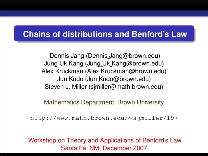
Chains of distributions and Benford’s Law Dennis Jang (Dennis Jang@brown.edu) Jung Uk Kang (Jung Uk Kang@brown.edu) Alex Kruckman (Alex Kruckman@brown.edu) Jun Kudo (Jun Kudo@brown.edu) Steven J. Miller (sjmiller@math.brown.edu) Mathematics Department, Brown University http://www.math.brown.edu/ ∼ sjmiller/197 Workshop on Theory and Applications of Benford’s Law Santa Fe, NM, December 2007 1
Problem Outline Alex Kossovsky conjectured that many chains of distributions approach Benford’s law. 2
Problem Outline Alex Kossovsky conjectured that many chains of distributions approach Benford’s law. Consider X 1 ∼ Unif ( 0 , k ) , X 2 ∼ Unif ( 0 , X 1 ) , ..., X n ∼ Unif ( 0 , X n − 1 ) . 3
Problem Outline Alex Kossovsky conjectured that many chains of distributions approach Benford’s law. Consider X 1 ∼ Unif ( 0 , k ) , X 2 ∼ Unif ( 0 , X 1 ) , ..., X n ∼ Unif ( 0 , X n − 1 ) . If f n , k ( x n ) is the probability density for X n , then � log n − 1 ( k / x n ) if x n ∈ [ 0 , k ] k Γ( n ) f n , k ( x n ) = 0 otherwise. 4
Problem Outline Alex Kossovsky conjectured that many chains of distributions approach Benford’s law. Consider X 1 ∼ Unif ( 0 , k ) , X 2 ∼ Unif ( 0 , X 1 ) , ..., X n ∼ Unif ( 0 , X n − 1 ) . If f n , k ( x n ) is the probability density for X n , then � log n − 1 ( k / x n ) if x n ∈ [ 0 , k ] k Γ( n ) f n , k ( x n ) = 0 otherwise. Theorem (JKKKM) As n → ∞ the distribution of digits of X n rapidly tends to Benford’s Law. 5
Uniform Density Example: n = 10 with 10,000 trials Digit Observed Probability Expected Probability 1 0.298 0.301 2 0.180 0.176 3 0.127 0.125 4 0.097 0.097 5 0.080 0.079 6 0.071 0.067 7 0.056 0.058 8 0.048 0.051 9 0.044 0.046 6
Sketch of the proof First prove the claim for density f n , k by induction. Use Mellin Transforms and Poisson Summation to analyze probability. 7
Proof by Induction: Base Case: Calculating CDF � k F 2 , k ( x 2 ) = Prob ( X 2 , k ∈ [ 0 , x 2 ] | X 1 , k = x 1 ) Prob ( X 1 , k = x 1 ) dx 1 0 8
Proof by Induction: Base Case: Calculating CDF � k F 2 , k ( x 2 ) = Prob ( X 2 , k ∈ [ 0 , x 2 ] | X 1 , k = x 1 ) Prob ( X 1 , k = x 1 ) dx 1 0 � x 2 Prob ( X 2 ∈ [ 0 , x 2 ] | X 1 = x 1 ) dx 1 = k 0 � k Prob ( X 2 ∈ [ 0 , x 2 ] | X 1 = x 1 ) dx 1 + k x 2 9
Proof by Induction: Base Case: Calculating CDF � k F 2 , k ( x 2 ) = Prob ( X 2 , k ∈ [ 0 , x 2 ] | X 1 , k = x 1 ) Prob ( X 1 , k = x 1 ) dx 1 0 � x 2 Prob ( X 2 ∈ [ 0 , x 2 ] | X 1 = x 1 ) dx 1 = k 0 � k Prob ( X 2 ∈ [ 0 , x 2 ] | X 1 = x 1 ) dx 1 + k x 2 � x 2 � k dx 1 x 2 dx 1 = x 2 k + x 2 log ( k / x 2 ) = + . k x 1 k k 0 x 2 10
Proof by Induction: Base Case: Calculating CDF � k F 2 , k ( x 2 ) = Prob ( X 2 , k ∈ [ 0 , x 2 ] | X 1 , k = x 1 ) Prob ( X 1 , k = x 1 ) dx 1 0 � x 2 Prob ( X 2 ∈ [ 0 , x 2 ] | X 1 = x 1 ) dx 1 = k 0 � k Prob ( X 2 ∈ [ 0 , x 2 ] | X 1 = x 1 ) dx 1 + k x 2 � x 2 � k dx 1 x 2 dx 1 = x 2 k + x 2 log ( k / x 2 ) = + . k x 1 k k 0 x 2 Differentiating yields f 2 , k ( x 2 ) = log ( k / x 2 ) . k 11
Further Comments Other distributions: exponential, one-sided normal. Weibull distribution: f ( x ; γ ) = γ x γ − 1 exp ( − x γ ) . Further areas of research - Two parameter distribution, closed form for other single variable distributions 12
Recommend
More recommend
Explore More Topics
Stay informed with curated content and fresh updates.
