
Carrier Phase and Symbol Timing Synchronization Saravanan - PowerPoint PPT Presentation
Carrier Phase and Symbol Timing Synchronization Saravanan Vijayakumaran sarva@ee.iitb.ac.in Department of Electrical Engineering Indian Institute of Technology Bombay November 2, 2012 1 / 28 The System Model Consider the following
Carrier Phase and Symbol Timing Synchronization Saravanan Vijayakumaran sarva@ee.iitb.ac.in Department of Electrical Engineering Indian Institute of Technology Bombay November 2, 2012 1 / 28
The System Model • Consider the following complex baseband signal s ( t ) K − 1 � s ( t ) = b i p ( t − iT ) i = 0 where b i ’s are complex symbols • Suppose the LO frequency at the transmitter is f c � √ 2 s ( t ) e j 2 π f c t � s p ( t ) = Re . • Suppose that the LO frequency at the receiver is f c − ∆ f • The received passband signal is y p ( t ) = As p ( t − τ ) + n p ( t ) • The complex baseband representation of the received signal is then y ( t ) = Ae j ( 2 π ∆ ft + θ ) s ( t − τ ) + n ( t ) 2 / 28
The System Model K − 1 y ( t ) = Ae j ( 2 π ∆ ft + θ ) � b i p ( t − iT − τ ) + n ( t ) i = 0 • Assume that the receiver side symbol rate is 1 + δ T • The unknown parameters are A , τ , θ , ∆ f and δ Timing Synchronization Estimation of τ Carrier Synchronization Estimation of θ and ∆ f Clock Synchronization Estimation of δ • Estimation approach depends on knowledge of b i ’s • Data-Aided Approach The b i ’s are known • The preamble of a packet contains known symbols • Decision-Directed Approach Decisions of b i ’s are used • Effective when symbol error rate is low • Non-Decision-Directed Approach The b i ’s are unknown • Averaging over the symbol distribution 3 / 28
Likelihood Function of Signals in AWGN • The likelihood function of signals in real AWGN is � 1 � y , s φ � − � s φ � 2 � �� L ( y | s φ ) = exp σ 2 2 • The likelihood function of signals in complex AWGN is � 1 Re ( � y , s φ � ) − � s φ � 2 � �� L ( y | s φ ) = exp σ 2 2 • Maximizing these likelihood functions as functions of φ results in the ML estimator 4 / 28
Carrier Phase Estimation • The change in phase due to the carrier offset ∆ f is 2 π ∆ fT in a symbol interval T • The phase can be assumed to be constant over multiple symbol intervals • Assume that the phase θ is the only unknown parameter • Assume that s ( t ) is a known signal in the following y ( t ) = s ( t ) e j θ + n ( t ) • The likelihood function for this scenario is given by � 1 Re ( � y , se j θ � ) − � se j θ � 2 � �� L ( y | s θ ) = exp σ 2 2 • Let � y , s � = Z = | Z | e j φ = Z c + jZ s � y , se j θ � e − j θ Z = | Z | e j ( φ − θ ) = Re ( � y , se j θ � ) = | Z | cos ( φ − θ ) � se j θ � 2 � s � 2 = 5 / 28
Carrier Phase Estimation • The likelihood function for this scenario is given by � 1 | Z | cos ( φ − θ ) − � s � 2 � �� L ( y | s θ ) = exp σ 2 2 • The ML estimate of θ is given by θ ML = φ = arg ( � y , s � ) = tan − 1 Z s ˆ Z c s c ( T − t ) Sampler at T × LPF y c ( t ) + s s ( T − t ) Sampler at T √ 2 cos 2 π f c t tan − 1 Z s ˆ y p ( t ) θ ML Z c √ − 2 sin 2 π f c t s c ( T − t ) Sampler at T − × y s ( t ) + LPF s s ( T − t ) Sampler at T 6 / 28
Phase Locked Loop • The carrier offset will cause the phase to change slowly • A tracking mechanism is required to track the changes in phase • For simplicity, consider an unmodulated carrier y p ( t ) = A cos ( 2 π f c t + θ ) + n ( t ) • The log likelihood function for this scenario is given by ln L ( y | s θ ) � y p ( t ) , A cos ( 2 π f c t + θ ) � − � A cos ( 2 π f c t + θ ) � 2 1 � � = σ 2 2 • For an observation interval T o , we get ˆ θ ML by maximizing Λ( θ ) = A � y p ( t ) cos ( 2 π f c t + θ ) dt σ 2 T o 7 / 28
Phase Locked Loop • A necessary condition for a maximum at ˆ θ ML is ∂ ∂θ Λ(ˆ θ ML ) = 0 • This implies � y p ( t ) sin ( 2 π f c t + ˆ θ ML ) dt = 0 T o � T o () dt y p ( t ) × VCO sin ( 2 π f c t + ˆ θ ) 8 / 28
Non-Decision-Directed PLL for BPSK • When the symbols are unknown we average the likelihood function over the symbol distribution • Suppose the transmitted signal is given by s ( t ) = A cos ( 2 π f c t + θ ) , 0 ≤ t ≤ T where A is equally likely to be ± 1. The likelihood function is given by �� T � �� r ( t ) s ( t ) dt − � s ( t ) � 2 1 L ( r | θ ) = exp σ 2 2 0 • Neglecting the energy of the signal as it is parameter independent we get the likelihood function � T � � 1 Λ( θ ) = exp r ( t ) s ( t ) dt σ 2 0 9 / 28
Non-Decision-Directed PLL for BPSK • We have to average Λ( θ ) over the distribution of A ¯ Λ( θ ) = E A [Λ( θ )] � T � � 1 1 = 2 exp r ( t ) cos ( 2 π f c t + θ ) dt σ 2 0 � T � � + 1 − 1 2 exp r ( t ) cos ( 2 π f c t + θ ) dt σ 2 0 � T � � 1 = cosh r ( t ) cos ( 2 π f c t + θ ) dt σ 2 0 10 / 28
Non-Decision-Directed PLL for BPSK • To find ˆ θ ML we can maximize ln ¯ Λ( θ ) instead of ¯ Λ( θ ) � T � � 1 ln ¯ Λ( θ ) = ln cosh r ( t ) cos ( 2 π f c t + θ ) dt σ 2 0 • Maximizing this function is difficult but approximations can be made which make the maximization easy x 2 � 2 , | x | ≪ 1 ln cosh x = | x | , | x | ≫ 1 • For an observation over K independent symbols � 2 � ( n + 1 ) T K − 1 � 1 ¯ � Λ K ( θ ) = exp r ( t ) cos ( 2 π f c t + θ ) dt σ 2 nT n = 0 11 / 28
Non-Decision-Directed PLL for BPSK A necessary condition on the ML estimate ˆ θ ML is � ( n + 1 ) T K − 1 � r ( t ) cos ( 2 π f c t + ˆ θ ML ) dt × nT n = 0 � ( n + 1 ) T r ( t ) sin ( 2 π f c t + ˆ θ ML ) dt = 0 nT � T () dt × Sampler at nT cos ( 2 π f c t + ˆ θ ) π 2 � K − 1 r ( t ) n = 0 () × VCO sin ( 2 π f c t + ˆ θ ) � × T () dt Sampler at nT 12 / 28
Costas Loop • Developed by Costas in 1956 × LPF cos ( 2 π f c t + ˆ θ ) π 2 Loop r ( t ) × VCO Filter sin ( 2 π f c t + ˆ θ ) × LPF • The received signal is r ( t ) = A ( t ) cos ( 2 π f c t + θ ) + n ( t ) = s ( t ) + n ( t ) 13 / 28
Costas Loop • The input to the loop filter is e ( t ) = y c ( t ) y s ( t ) where � � [ s ( t ) + n ( t )] cos ( 2 π f c t + ˆ y c ( t ) = θ ) LPF 1 2 [ A ( t ) + n i ( t )] cos ∆ θ + 1 = 2 n q ( t ) sin ∆ θ � � [ s ( t ) + n ( t )] sin ( 2 π f c t + ˆ y s ( t ) = LPF θ ) 1 2 [ A ( t ) + n i ( t )] sin ∆ θ − 1 = 2 n q ( t ) cos ∆ θ where n i ( t ) = LPF { n ( t ) cos ( 2 π f c t + θ ) } n q ( t ) = LPF { n ( t ) sin ( 2 π f c t + θ ) } 14 / 28
Costas Loop • The input to the loop filter is given by 1 � [ A ( t ) + n i ( t )] 2 − n 2 � e ( t ) = q ( t ) sin ( 2 ∆ θ ) 8 − 1 4 n q ( t ) [ A ( t ) + n i ( t )] cos ( 2 ∆ θ ) 1 8 A 2 ( t ) sin ( 2 ∆ θ ) + noise × signal + noise × noise = • The VCO output has a 180 ◦ ambiguity necessitating differential encoding of data 15 / 28
Symbol Timing Estimation • Consider the complex baseband received signal y ( t ) = As ( t − τ ) e j θ + n ( t ) where A , τ and θ are unknown and s ( t ) is known • For Γ = [ τ, θ, A ] the likelihood function is � 1 Re ( � y , s Γ � ) − � s Γ � 2 � �� L ( y | s Γ ) = exp σ 2 2 • For a large enough observation interval, the signal energy does not depend on τ and � s Γ � 2 = A 2 � s � 2 • For s MF ( t ) = s ∗ ( − t ) we have � Ae − j θ � y , s Γ � = y ( t ) s ∗ ( t − τ ) dt � Ae − j θ = y ( t ) s MF ( τ − t ) dt Ae − j θ ( y ⋆ s MF )( τ ) = 16 / 28
Symbol Timing Estimation • Maximizing the likelihood function is equivalent to maximizing the following cost function − A 2 � s � 2 � � Ae − j θ ( y ⋆ s MF )( τ ) J ( τ, A , θ ) = Re 2 • For ( y ⋆ s MF )( τ ) = Z ( τ ) = | Z ( τ ) | e j φ ( τ ) we have � � Ae − j θ ( y ⋆ s MF )( τ ) Re = A | Z ( τ ) | cos ( φ ( τ ) − θ ) • The maximizing value of θ is equal to φ ( τ ) • Substituting this value of θ gives us the following cost function J ( τ, A , θ ) = A | ( y ⋆ s MF )( τ ) | − A 2 � s � 2 J ( τ, A ) = argmax 2 θ 17 / 28
Symbol Timing Estimation • The ML estimator of the delay picks the peak of the matched filter output τ ML = argmax ˆ | ( y ⋆ s MF )( τ ) | τ s c ( − t ) × y c ( t ) + Squarer LPF s s ( − t ) √ 2 cos 2 π f c t Pick y p ( t ) + ˆ τ ML the peak √ − 2 sin 2 π f c t s c ( − t ) − × LPF y s ( t ) + Squarer s s ( − t ) 18 / 28
Decision-Directed Symbol Timing Tracking • For illustration, consider a baseband PAM signal 1 � r ( t ) = b i p ( t − iT − τ ) + n ( t ) i where τ is unknown and p ( t ) is known • Suppose the decisions on the b i ’s are correct • For s τ ( t ) = � i b i p ( t − iT − τ ) the likelihood function is � 1 � r , s τ � − � s τ � 2 � �� L ( r | s τ ) = exp σ 2 2 • For a large enough observation interval T o , the signal energy can be assumed to be independent of τ 1 Complex baseband case is only slightly different 19 / 28
Decision-Directed Symbol Timing Tracking • The ML estimate of τ is obtained by maximizing � Λ( τ ) = r ( t ) s τ ( t ) dt T o � � � = b i r ( t ) p ( t − iT − τ ) dt = b i y ( iT + τ ) T o i i where � y ( α ) = r ( t ) p ( t − α ) dt T o • A necessary condition on ˆ τ ML is d dy ( iT + ˆ τ ML ) � d τ Λ(ˆ τ ML ) = b i = 0 d τ i 20 / 28
Recommend


More recommend
Explore More Topics
Stay informed with curated content and fresh updates.