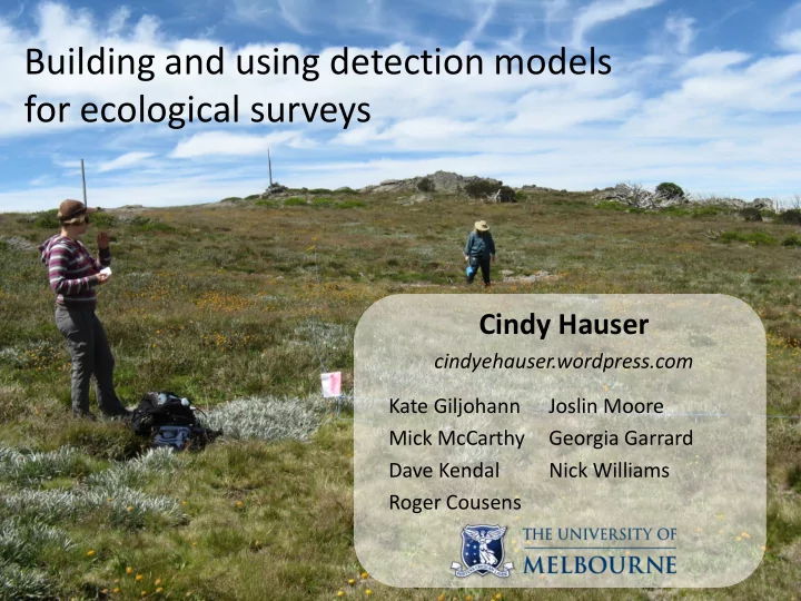
Building and using detection models for ecological surveys Cindy - PowerPoint PPT Presentation

Building and using detection models for ecological surveys Cindy Hauser cindyehauser.wordpress.com Kate Giljohann Joslin Moore Mick McCarthy Georgia Garrard Dave Kendal Nick Williams Roger Cousens

Ecological surveys • Is my species present or absent here? • How many individuals of my species are here? (abundance) • Where is my species located in the landscape? (distribution) • Walking (or swimming!) transects, standing at a point, looking or listening, using cameras, sound recorders, satellites or aircraft, traps, ...

Imperfect detection • What if my species is there but I don’t observe it? the study area was too big to survey all of it the frog was there but not calling the bird lives here but was foraging elsewhere the plant was hidden beneath a different, bigger plant I misidentified it as another species my species was there but I just failed to notice it • Survey designs need to take this into account

Hawkweeds in alpine Victoria http://en.wikipedia.org/wiki/Hawkweed http://flora.nhm-wien.ac.at/Seiten-Arten/Hieracium-praealtum-prae.htm http://www.ct-botanical-society.org/galleries/hieraciumpilo.html orange hawkweed King Devil hawkweed mouse-ear hawkweed Hieracium aurantiacum Hieracium praealtum Hieracium pilosella discovered 1999 discovered 2003 discovered 2011

Weed survey site weed weed absent present survey survey no detection detection no detection no control action no control action control action •survey •survey •survey •weed spread •control •(no spread)

Weed survey We aim to minimise expected impacts of a weed L ( x ) = p (1 - d ( x )) R probability of failing probability of consequences of to detect the weed weed presence detection failure using survey effort x Hauser C.E. & McCarthy M.A. 2009. Streamlining ‘search and destroy’: cost effective surveillance for invasive species management. Ecology Letters 12: 683—692.

Detection function d ( x ) 1 d ( x ) = 1 – exp(- λ x ) 0.9 detection probability 0.8 0.7 0.6 0.5 0.4 0.3 0.2 0.1 0 search effort, x

Survey/impact trade-off Minimise expected total cost of survey and impact T ( x ) = x + p (1 – d ( x )) R Optimal survey effort is  1 ≤ 0, pR  λ  =  * x ( ) λ ln pR  1 > pR  λ λ 

Optimal surveillance  1 ≤ 0, pR  λ  =  * x ( ) λ ln pR  1 > pR   λ λ pR is the expected impact of a detection failure 1/ λ is the average survey effort required to detect the weed if it’s present

Optimal surveillance ( ) λ ln pR 1 = > x * , pR λ λ optimal survey effort x* probability of weed presence p

Optimal surveillance ( ) λ ln pR 1 = > x * , pR λ λ optimal survey effort x* impact of an undetected weed R

Optimal surveillance ( ) λ ln pR 1 = > x * , pR λ λ optimal survey effort x* search efficiency λ

Spatial variation • We usually have a heterogeneous landscape • Varying… – probability of weed presence – ability to detect the weed – ability to control the weed – value of weed absence • Limited budget • How should we prioritise survey resources across such a space?

Survey budget Minimise expected impacts of the weed across all sites n ∑ ( ) = − L x x ( , ,..., x ) p 1 d x ( ) R 1 2 n i i i i = i 1 subject to a budget on search effort n ∑ = x B i = i 1

Optimal surveillance with a budget ( )  λ λ   ln p R ( ) k B + − =  i i i x k ( ) , i 1,..., k   = λ λ *    x k i i i  = +  0, i k 1,..., n where ( ) λ k ln p R 1 ∑ mean survey effort for each site, = i i i x k ( ) without a budget λ k = i 1 i k λ = mean survey efficiency ( ) k ∑ − k λ across sites 1 = i i 1

Optimal surveillance with a budget ( )  λ λ   ln p R ( ) k B + − =  i i i x k ( ) , i 1,..., k   = λ λ *    x k i i i  = +  0, i k 1,..., n ideal survey effort if we didn’t have a budget

Optimal surveillance with a budget ( )  λ λ   ln p R ( ) k B + − =  i i i x k ( ) , i 1,..., k   = λ λ *    x k i i i  = +  0, i k 1,..., n difference between ideal survey duration and what we have available per site

Optimal surveillance with a budget ( )  λ λ   ln p R ( ) k B + − =  i i i x k ( ) , i 1,..., k   = λ λ *    x k i i i  = +  0, i k 1,..., n adapt to take surveillance efficiency at this site into account

Occurrence modeling for p • Dominant wind directions from source orange hawkweed • Vegetation community • Wetness • Disturbance Williams, Hahs & Morgan. 2008. A dispersal-constrained habitat suitability model for predicting invasion of alpine vegetation. Ecological Applications 18: 347-359.

Orange hawkweed detection Probability of detection 1.0 0.8 0.6 d(x) 0.4 Low grassy 0.2 Shrubby 0.0 0 50 100 Search duration x (minutes/ha)

Orange hawkweed in the Victorian alps 0.000 – 0.003 0 – 1 low grassy 0.003 – 0.007 1 – 2.5 (easy to search) 0.007 – 0.014 2.5 – 5 shrubby 0.014 – 0.026 5 – 10 0.026 – 0.050 (difficult to search) 10 – 20 0 10km Map 1. Predicted probability of Map 2. Vegetation categories Map 3. Optimal search time orange hawkweed occurrence (minutes per 4ha site) Williams N.S.G., Hahs A.K. & Morgan J.W. 2008. A dispersal-constrained habitat suitability model for predicting invasion of alpine vegetation. Ecological Applications 18:347—359.

Hawkweed detection 1. Set up 20m x 20m plots 2. Hide hawkweeds in plots 3. Send searchers out find hawkweeds (and time them) 4. Interview searchers about their experience Hauser, Giljohann, Moore, McCarthy, Garrard & Kendal. In prep.

Detection models 1 p = 1 – exp(- λ x ) 0.9 detection probability, p 0.8 0.7 0.6 0.5 0.4 0.3 0.2 0.1 0 search effort, x ln( λ ijk ) = a + b 1 y 1 + b 2 y 2 +…

Hawkweed detection 1 Detection is influenced by... detection probability 0.8 • hawkweed appearance prior, grass 0.6 • hawkweed cluster size prior, heath 0.4 • hawkweed placement experiment, • dominant background 0.2 grass experiment, vegetation heath 0 0 2 4 6 8 10 • distracting yellow flowers survey effort (min/plot) • searcher experience • time since starting Experimental result assumes the searcher is at peak experience and time of day.

Detection extremes 1 Experienced person searches for flowering orange hawkweed in a grassy plot without competing yellow flowers, 3 hours in detection probability 0.8 0.6 0.4 Inexperienced person searches for flowering yellow hawkweed in a mixed grass/heath plot with high yellow flower coverage, early 0.2 0 0 10 20 30 40 50 60 survey effort (min/plot)

Ongoing research • We’ve found detection differences amongst rosettes, orange- flowering plants and yellow-flowering plants. How do we take these into account for survey design? • Detection varies in ways we can’t predict or control. How should we adapt surveys when our input parameters are uncertain? • How should we design a survey for multiple species? • How can we incorporate travel time into the optimisation?

Conclusions • Optimisation, decision theory and statistics have much to offer environmental management • Posing the problem and defining objectives can be challenging • Mathematics bridges the gap between ecologists’ observations and the true state of nature

Acknowledgements • ARC Linkage grant to Cousens, Williams & Duncan • Research team: Sacha Jellinek, Eric Ireland, Tracy Rout, Ellie Soh, Fran Alexander, Clare Brownridge Karen Herbert & Iris Curran • • Volunteer searchers • 2013 Winter School & IMB