Bounded Degree Spanning Tree using Iterative Relaxation Barna Saha - PowerPoint PPT Presentation

Bounded Degree Spanning Tree using Iterative Relaxation Barna Saha March 11, 2015

Bounded Degree Spanning Tree Iterative Minimum Spanning Tree Algorithm Iterative Algorithm for Degree Bounded Spanning Tree Primal Dual Methods for Algorithm Design

Problem Definition Problem We are given an undirected graph G = ( V , E ) with a degree upper bound B v on each vertex v, and cost on edges c : E → R + . The task is to find a minimum cost spanning tree which satisfies all the degree bounds. ◮ The problem is NP-hard. Since, if every node has degree upper bound 2, and we can solve it exactly then we know whether the graph G has a hamiltonian path or not. ◮ We will show an algorithm which returns a spanning tree T of cost at most OPT where d T ( v ) ≤ B v + 1 for all v , where d T ( v ) denotes the degree of v in T .

Spanning Tree Polytope with Degree Bounds ◮ Given a subset S ⊆ V , we use E ( S ) to denote all edges with two end points in S . ◮ We use δ ( S ) to denote all edges with exactly one end point in S Here is the natural LP relaxation. � minimize c ( x ) = c e x e (1) e ∈ E subject to x ( E ( V )) = | V | − 1 (2) x ( E ( S )) ≤ | S | − 1 ∀ S ⊂ V (3) x ( δ ( v )) ≤ B v ∀ v ∈ V (4) x e ≥ 0 ∀ e ∈ E (5) We can solve this LP using ellipsoid method, as there exists a polynomial time separation oracle (Read chapter 11.2 of Shmoys and Williamson)

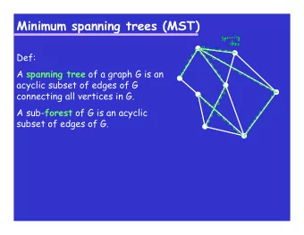
Spanning Tree Polytope � minimize c ( x ) = c e x e (LP-MST) e ∈ E subject to x ( E ( V )) = | V | − 1 (6) x ( E ( S )) ≤ | S | − 1 ∀ S ⊂ V (7) x e ≥ 0 ∀ e ∈ E (8) We will first show an iterative procedure to obtain a minimum spanning tree of G .

Iterative Minimum Spanning Tree Algorithm ◮ Initialization F ← φ ◮ While V ( G ) � = φ do ◮ Find a basic optimal solution x ∗ of LP-MST( G ) and remove every edge e with x ∗ e = 0 from G . ◮ Find a vertex v with at most one edge e = uv incident at it, and update F → F ∪ { e } , G → G \ { v } . ◮ Return F

Proof: Step 1 Lemma If the Iterative MST Algorithm terminates then the algorithm returns an optimal solution. Proof. If the algorithm finds a degree 1 vertex v , then x ( δ ( v )) ≥ 1. Hence if edge e = ( u , v ) incident on v , x ∗ e = 1. x ( E ( S )) = | V | − 1 , x ( E ( S \ v )) ≤ | V | − 1 − 1 = | V | − 2 . x ( δ ( v )) = x ( E ( S )) − x ( E ( S \ v )) ≥ 1 ◮ Given any spanning tree T ′ of G ′ = G \ { v } , T ′ ∪ { e } is a spanning tree of G . ◮ Solve the problem recursively on G ′ .

Proof: Step 1 Lemma If the Iterative MST Algorithm terminates then the algorithm returns an optimal solution. ◮ Solve the problem recursively on G ′ . ◮ Restriction of x ∗ to G ′ (denoted x ∗ res ) is a feasible solution for LP-MST( G ′ ). ◮ Inductively, we have an optimal solution F ′ for G ′ . ◮ Hence, if F is the final solution, F = F ′ ∪ e . c ( F ) = c ( F ′ ) + c e ≤ c ( x ∗ res ) + c e = c ( x ∗ )

Proof: Step 2 Lemma For any basic solution x ∗ of LP-MST ( G ) with support E ∗ = { e | x ∗ e > 0 } , there exists a vertex v with deg E ∗ ( v ) = 1 ◮ Proof Sketch ◮ Show there are at most | V | − 1 linearly independent tight constraints. ◮ By definition of basic solution, this implies there are at most | V | − 1 edges with fractional values. ◮ This implies there exists one vertex with degree 1.

Proof: Step 2 Lemma For any basic solution x ∗ of LP-MST ( G ) with support E ∗ = { e | x ∗ e > 0 } , there exists a vertex v with deg E ∗ ( v ) = 1 ◮ Proof Sketch ◮ Show there are at most | V | − 1 linearly independent tight constraints. ◮ By definition of basic solution, this implies there are at most | V | − 1 edges with fractional values. ◮ This implies there exists one vertex with degree 1.

Proof: Step 2: Notations ◮ Let F = { S | x ∗ ( E ( S )) = | S | − 1 } be the set of tight constraints. ◮ For a set S ⊆ V , the corresponding constraint x ∗ ( E ( S )) ≤ | S | − 1 defines a vector in R | E | : the vector has a 1 corresponding to each edge e ∈ E ( S ), and 0 otherwise. ◮ characteristic vector of E ( S ): denoted X E ( S )

Proof: Step 2: Notations ◮ Let F = { S | x ∗ ( E ( S )) = | S | − 1 } be the set of tight constraints. ◮ For a set S ⊆ V , the corresponding constraint x ∗ ( E ( S )) ≤ | S | − 1 defines a vector in R | E | : the vector has a 1 corresponding to each edge e ∈ E ( S ), and 0 otherwise. ◮ characteristic vector of E ( S ): denoted X E ( S ) ◮ span ( F ): vector space generated by linear combination of vectors {X E ( S ) | S ∈ F}

Proof: Step 2: Notations ◮ Let F = { S | x ∗ ( E ( S )) = | S | − 1 } be the set of tight constraints. ◮ For a set S ⊆ V , the corresponding constraint x ∗ ( E ( S )) ≤ | S | − 1 defines a vector in R | E | : the vector has a 1 corresponding to each edge e ∈ E ( S ), and 0 otherwise. ◮ characteristic vector of E ( S ): denoted X E ( S ) ◮ span ( F ): vector space generated by linear combination of vectors {X E ( S ) | S ∈ F} ◮ Two sets X and Y are intersecting, if X ∩ Y , X − Y , Y − X are nonempty. A family of sets is laminar if no two sets are intersecting.

Proof: Step 2: Notations ◮ Let F = { S | x ∗ ( E ( S )) = | S | − 1 } be the set of tight constraints. ◮ For a set S ⊆ V , the corresponding constraint x ∗ ( E ( S )) ≤ | S | − 1 defines a vector in R | E | : the vector has a 1 corresponding to each edge e ∈ E ( S ), and 0 otherwise. ◮ characteristic vector of E ( S ): denoted X E ( S ) ◮ span ( F ): vector space generated by linear combination of vectors {X E ( S ) | S ∈ F} ◮ Two sets X and Y are intersecting, if X ∩ Y , X − Y , Y − X are nonempty. A family of sets is laminar if no two sets are intersecting. ◮ We can obtain a laminar family L ⊆ F such that span ( L ) = span ( F ).

Proof: Step 2 ◮ Show there are at most | V | − 1 linearly independent tight constraints. ◮ Show |L| ≤ | V | − 1 where each S ∈ L has cardinality at least 2. ◮ Show by induction. There are | V | ground elements. The size of a laminar family each having cardinality at least 2 is bounded by | V | − 1.

Proof: Step 2 Show a laminar family L exists with span ( L ) = span ( F ) .

Lemma If S , T ∈ F and S ∩ T � = φ , then both S ∩ T and S ∪ T are in F . Furthermore, X E ( S ) + X E ( T ) = X E ( S ∩ T ) + X E ( S ∪ T ) . ◮ Implies the 4 constraints corresponding to S , T , S ∪ T , S ∩ T are not all tight and linearly independent. ◮ We do not need to consider (say) T . ◮ We therefore have three laminar constraints.

Proof: Step 2 Lemma If S , T ∈ F and S ∩ T � = φ , then both S ∩ T and S ∪ T are in F . Furthermore, X E ( S ) + X E ( T ) = X E ( S ∩ T ) + X E ( S ∪ T ) . Proof. As S ∩ T � = φ , we have: | S | − 1 + | T | − 1 = | S ∩ T | − 1 + | S ∪ T | − 1 ( | S | + | T | − | S ∩ T | = | S ∪ T | ) ≥ x ∗ ( E ( S ∩ T )) + x ∗ ( E ( S ∪ T )) ( x ∗ ( E ( S )) ≤ | S | − 1 for all S ⊂ V ) ≥ x ∗ ( E ( S )) + x ∗ ( E ( T )) (not counting edges that go from S to T ) = | S | − 1 + | T | − 1 used x ∗ ( E ( S )) = | S | − 1 , x ∗ ( E ( T )) = | T | − 1 All inequalities must be equalities.

Proof: Step 2 Lemma If S , T ∈ F and S ∩ T � = φ , then both S ∩ T and S ∪ T are in F . Furthermore, X E ( S ) + X E ( T ) = X E ( S ∩ T ) + X E ( S ∪ T ) . Proof. As S ∩ T � = φ , we have: | S | − 1 + | T | − 1 = | S ∩ T | − 1 + | S ∪ T | − 1 ( | S | + | T | − | S ∩ T | = | S ∪ T | ) ≥ x ∗ ( E ( S ∩ T )) + x ∗ ( E ( S ∪ T )) ( x ∗ ( E ( S )) ≤ | S | − 1 for all S ⊂ V ) ≥ x ∗ ( E ( S )) + x ∗ ( E ( T )) (not counting edges that go from S to T ) = | S | − 1 + | T | − 1 used x ∗ ( E ( S )) = | S | − 1 , x ∗ ( E ( T )) = | T | − 1 Constraints for S ∪ T and S ∩ T are also tight. x ∗ ( E ( S ∪ T )) = | S ∪ T | − 1 , and x ∗ ( E ( S ∩ T )) = | S ∩ T | − 1

Proof: Step 2 Lemma If S , T ∈ F and S ∩ T � = φ , then both S ∩ T and S ∪ T are in F . Furthermore, X E ( S ) + X E ( T ) = X E ( S ∩ T ) + X E ( S ∪ T ) . Proof. As S ∩ T � = φ , we have: | S | − 1 + | T | − 1 = | S ∩ T | − 1 + | S ∪ T | − 1 ( | S | + | T | − | S ∩ T | = | S ∪ T | ) ≥ x ∗ ( E ( S ∩ T )) + x ∗ ( E ( S ∪ T )) ( x ∗ ( E ( S )) ≤ | S | − 1 for all S ⊂ V ) ≥ x ∗ ( E ( S )) + x ∗ ( E ( T )) (not counting edges that go from S to T ) = | S | − 1 + | T | − 1 used x ∗ ( E ( S )) = | S | − 1 , x ∗ ( E ( T )) = | T | − 1 No edge from S to T . Hence X E ( S ) + X E ( T ) = X E ( S ∩ T ) + X E ( S ∪ T ) .

Proof: Step 2 Lemma If L is a maximal laminar subfamily of F , then span ( L ) = span ( F ) Proof. ◮ Suppose S ∈ F but X E ( S ) / ∈ span ( L ). Choose one such S that intersects as few sets of L as possible. ◮ Let S ∩ T � = φ and T ∈ L ◮ We have S ∩ T and S ∪ T are in F , but both of them are not in L , otherwise S will be in span ( F ). ◮ Both S ∪ T and S ∩ T intersects fewer sets in L than S –contradiction.

Iterative Algorithm for Degree Bounded Spanning Tree In the following we assume degree bounds are only given for vertices in W . � minimize c ( x ) = c e x e (LP-MBDST) e ∈ E subject to x ( E ( V )) = | V | − 1 (Type-1) x ( E ( S )) ≤ | S | − 1 ∀ S ⊂ V (Type-2) x ( δ ( v )) ≤ B v ∀ v ∈ W (Type-Degree) x e ≥ 0 ∀ e ∈ E (9) Initially W = V