Minimum Spanning Tree Given a connected graph, we often want the - PowerPoint PPT Presentation

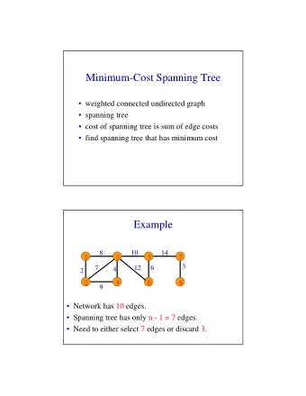
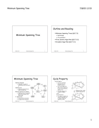
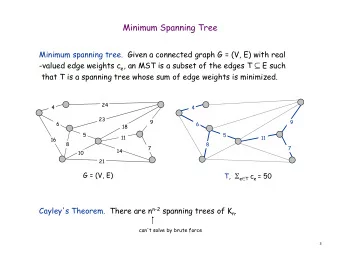
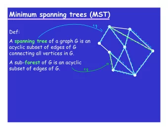
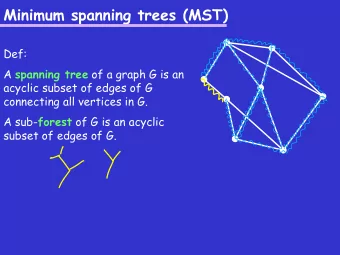
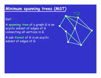
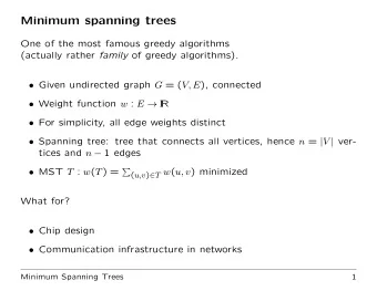
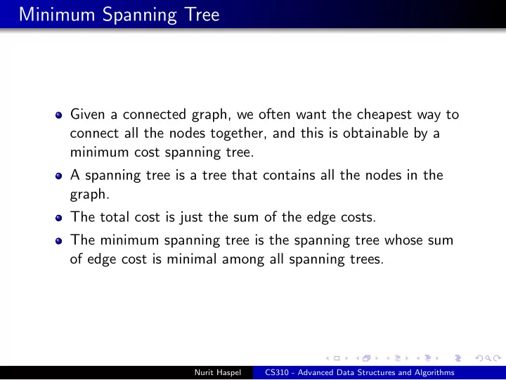
Minimum Spanning Tree Given a connected graph, we often want the cheapest way to connect all the nodes together, and this is obtainable by a minimum cost spanning tree. A spanning tree is a tree that contains all the nodes in the graph. The total cost is just the sum of the edge costs. The minimum spanning tree is the spanning tree whose sum of edge cost is minimal among all spanning trees. Nurit Haspel CS310 - Advanced Data Structures and Algorithms

Minimum Spanning Tree The kind of tree involved here has no particular root node, and such trees are called free trees, because they are not tied down by a root. Weiss relates the min-cost spanning tree problem to the Steiner tree problem. If you want to see an example of a Steiner tree, follow this link: http://www.cs.sunysb.edu/~algorith/files/ steiner-tree.shtml Nurit Haspel CS310 - Advanced Data Structures and Algorithms

Kruskal’s algorithm This algorithm is a lot like Huffman’s. Start with all the nodes separate and then stick them together incrementally, using a greedy approach that turns out to give you the optimal solution. Set up a partition, a set of sets of nodes, starting with one node in each set. Then find the minimal edge to join two sets, and use that as a tree edge, and join the sets. Nurit Haspel CS310 - Advanced Data Structures and Algorithms

Example 2 2 v 0 v 1 v 0 v 1 10 4 3 1 1 2 2 v 2 v 3 v 4 v 2 v 3 v 4 2 2 4 4 8 5 6 v 5 v 6 v 5 v 6 1 1 Nurit Haspel CS310 - Advanced Data Structures and Algorithms

Example v 0 v 1 v 0 v 1 1 1 v 2 v 3 v 4 v 2 v 3 v 4 v 5 v 6 v 5 v 6 1 2 1 2 2 v 0 v 1 v 0 v 1 1 1 v 2 v 3 v 4 v 2 v 3 v 4 2 v 5 v 6 v 5 v 6 3 4 1 1 Nurit Haspel CS310 - Advanced Data Structures and Algorithms

Example 2 2 v 0 v 1 v 0 v 1 3 1 1 2 2 v 2 v 3 v 4 v 2 v 3 v 4 2 2 v 5 v 6 v 5 v 6 5 6 1 1 2 2 v 0 v 1 v 0 v 1 4 1 1 2 2 v 2 v 3 v 4 v 2 v 3 v 4 2 2 4 v 5 v 6 v 5 v 6 7 8 1 1 Nurit Haspel CS310 - Advanced Data Structures and Algorithms

Kruskal’s Algorithm Note that several edges are left unprocessed in the edge list: these are the high-cost edges we were hoping to avoid using. Implementation: There are fancy data structures for partitions. Come back to this chapter if you ever need to do this with good performance. In cases that don’t need the very best performance, a Map from vertex to partition number will do the job of holding the partition. Nurit Haspel CS310 - Advanced Data Structures and Algorithms

Running Example Here are the partition numbers for the first few steps: Node V 0 V 1 V 2 V 3 V 4 V 5 V 6 Set 0 1 2 3 4 5 6 V 0 - V 3 0 1 2 0 4 5 6 (3s turned into 0s) V 5 - V 6 0 1 2 0 4 5 5 (6s turned into 5s) V 0 - V 1 0 0 2 0 4 5 5 V 2 - V 3 0 0 0 0 4 5 5 and so on. Edges are used in cost order. If an edge has both to and from vertices with the same partition number, it is skipped. The resulting tree is defined by the edges used. Nurit Haspel CS310 - Advanced Data Structures and Algorithms

Prim’s algorithm for MST Quite similar to Kruskal: Initialize tree V=v s.t. v is an arbitrary node. Initialize E= {} . Repeat until all nodes are in T: Choose an edge e=(v,w) with minimum weight such that v is in T and w is not. Add w to T, add e to E. Output T=(V,E) Nurit Haspel CS310 - Advanced Data Structures and Algorithms

Greedy Choice Property Both greedy algorithms are optimal. That is – they guarantee to give an MST. The greedy choice here is to always select a lightest edge e we can still use (there may be more than one). (Somewhat sketchy proof:) Suppose we do not select e = ( u , v ), a lightest edge we can select at some point. Then there is a path in T from u to v , and this path does not contain the edge ( u , v ) by assumption. Since when we could select e , u and v were not on the same component, there must be some edge on the path we could still select instead of e . Say this edge is e ′ = ( x , y ). Now let us remove the edge e = ( x , y ) from the MST T . This breaks T into two components, one containing u and one containing v . Nurit Haspel CS310 - Advanced Data Structures and Algorithms

Greedy Choice Property Now let us add the edge ( u , v ). This reattaches those two components and creates a new spanning tree T ′ . We have w ( T ′ ) = w ( T ) − w ( x , y ) + w ( u , v ) ≤ w ( T ) (because e = ( u , v ) is a lightest edge we can select at that stage). Corollary: Every MST contains the lightest edge in the graph (as a matter of fact, as many of them as we can add w/o closing a cycle). Nurit Haspel CS310 - Advanced Data Structures and Algorithms