
CPSC 490 Problem Solving in Computer Science Trees, MST, Euler - PowerPoint PPT Presentation
CPSC 490 Problem Solving in Computer Science Trees, MST, Euler Tour, and Backtracking Lucca Siaudzionis and Jack Spalding-Jamieson 2020/01/16 University of British Columbia Announcements Office hours will be Tuesdays from 2-4pm in ICCS
CPSC 490 Problem Solving in Computer Science Trees, MST, Euler Tour, and Backtracking Lucca Siaudzionis and Jack Spalding-Jamieson 2020/01/16 University of British Columbia
Announcements • Office hours will be Tuesdays from 2-4pm in ICCS X237. • After today’s lecture, you will be able to solve all but a few of the A1 problems. • If you’re having any trouble with the basics (piazza, assignment submissions, IO, etc.), please ask after class. 1
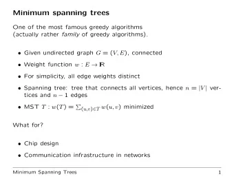
What is a Tree? A Tree is a graph with: • Exactly N − 1 edges (with N nodes) • A path between every pair of nodes 2
Trees’ Properties • There is exactly one path between each pair of nodes • There are no cycles (you can try to prove this!) • It is sparse (i.e. there are very few edges) 3
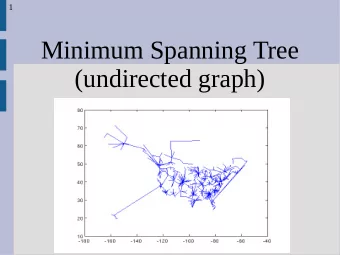
Spanning Tree Given a Graph G , a Spanning Tree is a tree within the original graph that contains all its nodes 4
Minimum/Maximum Spanning Trees Given a Graph G , a minimum/maximum spanning tree is a tree within the original graph that • Is a spanning tree • Sum of the weights is minimized/maximized 5
Minimum Spanning Tree 5 8 8 4 10 2 5 6
Finding Some Spanning Tree An intuitive way to build a spanning tree: • Start with an empty tree • Iterate through all the edges • Given an edge ( x , y ) • If x and y are connected (i.e. there is already a path from x to y ), ignore this edge • Otherwise, add this edge to the tree 7
Kruskal’s Algorithm for MST Sort the edges by weight • Ascending weight if Minimum ST • Descending weight if Maximum ST Then, do what we did before: • Start with an empty tree • Iterate through all the edges in sorted order • Given an edge ( x , y ) • If x and y are connected (i.e. there is already a path from x to y ), ignore this edge • Otherwise, add this edge to the tree 8
Kruskal’s Algorithm Illustrated 9 3 11 6 10 12 7 8 9
Kruskal’s Algorithm Illustrated 9 3 11 6 10 12 7 8 10
Kruskal’s Algorithm Illustrated 9 3 11 6 10 12 7 8 11
Kruskal’s Algorithm Illustrated 9 3 11 6 10 12 7 8 12
Kruskal’s Algorithm Illustrated 9 3 11 6 10 12 7 8 13
Kruskal’s Algorithm Illustrated 9 3 11 6 10 12 7 8 14
Kruskal’s Algorithm Illustrated 9 3 11 6 10 12 7 8 15
Kruskal’s Algorithm Illustrated 9 3 11 6 10 12 7 8 16
Kruskal’s Algorithm Illustrated 9 3 11 6 10 12 7 8 17
Kruskal’s Algorithm Illustrated 9 3 11 6 10 12 7 8 18
Kruskal’s Algorithm Illustrated 9 3 11 6 10 12 7 8 19
Kruskal’s Algorithm Illustrated 9 3 11 6 10 12 7 8 20
Kruskal’s Algorithm Illustrated 9 3 11 6 10 12 7 8 21
Kruskal’s Algorithm Illustrated 9 3 11 6 10 12 7 8 22
Kruskal’s Algorithm Illustrated 9 3 11 6 10 12 7 8 This is the resulting Minimum Spanning Tree. 23
Kruskal’s Algorithm - Connectivity Sort the edges by weight • Ascending weight if Minimum ST • Descending weight if Maximum ST Then, do what we did before: • Start with an empty tree • Iterate through all the edges in sorted order • Given an edge ( x , y ) • If x and y are connected (i.e. there is already a path from x to y ), ignore this edge • Otherwise, add this edge to the tree 24
Kruskal’s Algorithm - Connectivity How do we find out with vertices x and y are already connected by the edges chosen so far? • Slow Idea: Run a traversal (DFS or BFS) from node x • This would cost O (#Edges picked so far) • Hence, iterating through all edges would cost O ( N × M ), which is too slow 25
Kruskal’s Algorithm - Connectivity How do we find out with vertices x and y are already connected by the edges chosen so far? • Fast Idea: Use Union-Find • Checking whether two objects are part of the same component using Union-Find is very fast (essentially O (1) 1 ) • Hence, iterating through all edges would cost O ( M ) 1 Technically, it is not O (1). However, it is fast enough that we can pretend it is. 26
Kruskal’s Algorithm - Complexity Sort the edges by weight – O ( M log M ) • Ascending weight if Minimum ST • Descending weight if Maximum ST Then, do what we did before: • Start with an empty tree • Iterate through all the edges in sorted order – O ( M ) • Given an edge ( x , y ) • If x and y are connected (i.e. there is already a path from x to y ), ignore this edge – O(1) • Otherwise, add this edge to the tree Algorithm Complexity: O ( M log M ) 27
Discussion Problem Input: Given N cities. You are tasked to connect these cities with roads using ( N − 1) edges. Two construction companies made proposals to build roads. Each proposal specifies two cities the road would connect and the road’s cost. You were bribed to give exactly K contracts to company A. Output: Minimum total cost to connect all cities under those requirements. Constraints: 0 < N < 50 , 000, 0 ≤ K < N . 28
Discussion Problem - Insight Choose exactly N − 1 roads with minimum cost → MST! But simply running MST cannot guarantee exactly K roads from company A. Solution: • Pick a penalty/incentive P for MST • Add P to the cost of each road proposed by company A • Run MST • MST didn’t choose K roads from company A? Tweak P and try again! • Binary search on P 29
The n - k Queens Problem Input : An n × n -sized chessboard, and k queen pieces. Output : Is there a placement of all the queen pieces so that no piece can attack any other? That is: No two pieces share a row, column, or diagonal. An example for 8 queens on an 8 by 8 board. (image from en.wikipedia.org/wiki/Eight queens puzzle) 30
The n - k -Queens Problem, More General We can solve an even harder problem! Input : An n × n chessboard, and k queen pieces. Output : The number of placements where all the queen pieces cannot attack each other. Note: We say two placements are different if the set of positions is different. However, in this case is it equivalent (in some sense) to say that the exact placement of some named queen is different, since this multiplies our number of solutions by n !. 31
The n - k -Queens Problem, Backtracking Approach (1) The easiest brute force method for this problem is to try every placement of the pieces. We can do this recursively: 21 int nkqueens(vector<vector<int>> &cur_placements, int n, int k) { if (k <= 0) return 1; 22 int ans = 0; 23 for (int i = 0; i < n; ++i) for (int j = 0; j < n; ++j) 24 if (cur_placements[i][j] == 0) { 25 set_rcd(cur_placements,n,i,j,1); //place & block rcd 26 ans += nkqueens(cur_placements, n, k-1); 27 set_rcd(cur_placements,n,i,j,-1); //undo blocks 28 } 29 return ans; 30 31 } 32 int nkqueens(int n, int k) { vector<vector<int>> cur_placements(n,vector<int>(n)); 33 return nkqueens(cur_placements, n, k)/factorial(n); // note: need to implement factorial 34 35 } 32
The n - k -Queens Problem, Backtracking Approach (2) 1 // set row, column, and diagonal around point (i,j) to v 2 void set_rcd(vector<vector<int>> &b, int n, int i, int j, int v) { for (int k = 0; k < n; ++k) { 3 b[k][j] += v; 4 b[i][k] += v; 5 } 6 int i_pos = i, j_pos = j; 7 while (i_pos >= 0 && j_pos >= 0) { 8 --i_pos; --j_pos; 9 } 10 for (++i_pos, ++j_pos; i_pos < n && j_pos < n; ++i_pos, ++j_pos) 11 b[i_pos][j_pos] += v; 12 int i_neg = i, j_neg = j; 13 while (i_neg >= 0 && j_neg < n) { 14 --i_neg; ++j_neg; 15 } 16 for (++i_neg, --j_neg; i_neg < n && j_neg >= 0; ++i_neg, --j_neg) 17 b[i_neg][j_neg] += v; 18 19 } 33
The n - k -Queens Problem, Analysis The brute force code uses O ( n 2 ) memory, and runs in O (( n 2 ) k ) time. Our run-time for our code is exponential. However, in practice, it is very fast.It is part of a more general approach, called Backtracking , which has some characteristics that make it fast in practice. 34
Backtracking - Pseudocode Backtracking is very general solution approach that matches the following code template: fun backtrack(candidate): 1 if candidate is a complete solution: 2 return 1 3 num_soln = 0 4 for every valid next extension of candidate: 5 make the extension , and record this in candidate 6 num_soln += backtrack(candidate) 7 undo the extension 8 return num_soln 9 10 create an empty candidate solution S 11 backtrack(S) 12 35
Backtracking - Boolean Version This can also be altered slightly to simply determine if a solution exists at all: fun backtrack(candidate): 1 if candidate is a complete solution: 2 return true 3 for every valid next extension of candidate: 4 make the extension , and record this in candidate 5 if backtrack(candidate): 6 return true; 7 undo the extension 8 return false 9 10 create an empty candidate solution S 11 backtrack(S) 12 36
Recommend


More recommend
Explore More Topics
Stay informed with curated content and fresh updates.