The scaling limit of the MST of a complete graph Nicolas Broutin, - PowerPoint PPT Presentation

The scaling limit of the MST of a complete graph Nicolas Broutin, Inria Paris-Rocquencourt joint work with L. Addario-Berry, McGill C. Goldschmidt, Oxford G. Miermont, ENS Lyon

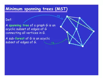
The minimum spanning tree Definition. G = ( V , E ) a connected graph w e ≥ 0 , e ∈ E weights MST = lightest connected subgraph of G Kruskal’s algorithm. 1. sort the edges by increasing weight, e i , 1 ≤ i ≤ | E | 2. Initially set T 0 = ( V , ∅ ) 3. Set T i +1 = T i ∪ { e i } iff it does not create a cycle

Kruskal – Example 1 4 10 7 3 6 2 8 9 5

Kruskal – Example 1 4 10 7 3 6 2 8 9 5

Kruskal – Example 1 4 10 7 3 6 2 8 9 5

Kruskal – Example 1 4 10 7 3 6 2 8 9 5

Kruskal – Example 1 4 10 7 3 6 2 8 9 5

Kruskal – Example 1 4 10 7 3 6 2 8 9 5

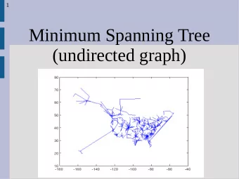
Random Model ”Mean-field” model graph: complete graph K n weights: iid uniform A little history. Frieze (’85): total weight converges to ζ (3) Janson (’95): CLT Aldous: degree of the node 1

Random Model ”Mean-field” model graph: complete graph K n weights: iid uniform A little history. Frieze (’85): total weight converges to ζ (3) Janson (’95): CLT Aldous: degree of the node 1 But... all these informations are local What is the global metric structure?

The continuum spanning tree The rescaled minimum spanning tree • T n the minimum spanning tree of K n • n − 1 / 3 d n , for d n the graph distance • µ n mass n − 1 on each vertex Theorem (ABGM ’13) There exists a random compact metric space M s.t. d − − − → T n GHP M

Comparing metric spaces Gromov-Hausdorff topology. ( X 1 , d 1 ) ( X 2 , d 2 ) φ 1 φ 2 ( Z , δ )

Comparing measured metric spaces Gromov-Hausdorff-Prokhorov topology. ( X 1 , d 1 , µ 1 ) ( X 2 , d 2 , µ 2 ) φ 1 φ 2 ( Z , δ )

What does it look like? M

A few properties of M Proposition. 1. M is a tree-like metric space 2. M has maximum degree 3 3. for µ -almost every x , deg( x ) = 1

A few properties of M Proposition. 1. M is a tree-like metric space 2. M has maximum degree 3 3. for µ -almost every x , deg( x ) = 1 Proposition. M is not Aldous’ Continuum Random Tree (CRT)

Elements of proof Random graphs Phase transition Scaling limit of large trees / CRT Structure of critical random graphs Minimum spanning tree

G ( n , p ) random graphs Definition. Random graph G ( n , p ) graph on { 1 , 2 , . . . , n } independently, take edges with probability p C n i the connected components in decreasing order of size Phase transition: G ( n , c / n ) | C n c < 1: 1 | = O (log n ) k | ≈ n 2 / 3 | C n 1 | , | C n 2 | , . . . , | C n c = 1: | C n | C n c > 1: 1 | = Ω( n ), 2 | = O (log n )

The phase transition in pictures

The phase transition in pictures 1 . 0 G (10000 , 10000 )

The phase transition in pictures

When is the metric structure built? T ( n , p ) portion of the MST that is in G ( n , p ) T ( n , p ) = ( T 1 ( n , p ) , T 2 ( n , p ) , . . . ) Evolution of distances: • for all p < (1 − ǫ ) / n d GH ( T ( n , p ); “empty graph”) = O (log n ) • for all p > (1 + ǫ ) / n d GH ( T 1 ( n , p ); MST ) = O (log 10 n )

When is the metric structure built? T ( n , p ) portion of the MST that is in G ( n , p ) T ( n , p ) = ( T 1 ( n , p ) , T 2 ( n , p ) , . . . ) Evolution of distances: • for all p < (1 − ǫ ) / n d GH ( T ( n , p ); “empty graph”) = O (log n ) • for all p > (1 + ǫ ) / n d GH ( T 1 ( n , p ); MST ) = O (log 10 n ) Look around the critical phase p ⋆ = 1 / n + λ n − 4 / 3 λ ∈ R large

The phase transition For np = 1 + λ n − 1 / 3 Theorem. (Aldous ’97) λ ∈ R ( n − 2 / 3 | C n i | , s ( C n i )) i ≥ 1 → ( | γ i | , s ( γ i )) i ≥ 1

The phase transition For np = 1 + λ n − 1 / 3 Theorem. (Aldous ’97) λ ∈ R ( n − 2 / 3 | C n i | , s ( C n i )) i ≥ 1 → ( | γ i | , s ( γ i )) i ≥ 1 W Brownien W λ t = λ t − t 2 / 2 + W t B λ t = W λ t − inf s ≤ t W λ t

The phase transition For np = 1 + λ n − 1 / 3 Theorem. (Aldous ’97) λ ∈ R ( n − 2 / 3 | C n i | , s ( C n i )) i ≥ 1 → ( | γ i | , s ( γ i )) i ≥ 1 W Brownien W λ t = λ t − t 2 / 2 + W t B λ t = W λ t − inf s ≤ t W λ t

The phase transition For np = 1 + λ n − 1 / 3 Theorem. (Aldous ’97) λ ∈ R ( n − 2 / 3 | C n i | , s ( C n i )) i ≥ 1 → ( | γ i | , s ( γ i )) i ≥ 1 W Brownien W λ t = λ t − t 2 / 2 + W t B λ t = W λ t − inf s ≤ t W λ t

The phase transition For np = 1 + λ n − 1 / 3 Theorem. (Aldous ’97) λ ∈ R ( n − 2 / 3 | C n i | , s ( C n i )) i ≥ 1 → ( | γ i | , s ( γ i )) i ≥ 1 W Brownien s ( γ ) W λ t = λ t − t 2 / 2 + W t B λ t = W λ t − inf s ≤ t W λ t Poisson rate 1 on R 2 + | γ |

The tree encoded by an excursion 0 1 excursion f tree T f For a continuous excursion f Definition: d f ( x , y ) = f ( x ) + f ( y ) − 2 x ∧ y ≤ t ≤ x ∨ y f ( t ) inf x ∼ f y if d f ( x , y ) = 0 ([0 , 1] / ∼ f , d f ) is a tree-like metric space

The tree encoded by an excursion 0 1 excursion f tree T f For a continuous excursion f Definition: d f ( x , y ) = f ( x ) + f ( y ) − 2 x ∧ y ≤ t ≤ x ∨ y f ( t ) inf x ∼ f y if d f ( x , y ) = 0 ([0 , 1] / ∼ f , d f ) is a tree-like metric space

Aldous’ Continuum Random Tree (CRT) Theorem. (Aldous ’91) T n a uniformly random tree on { 1 , 2 , . . . , n } d n − 1 / 2 T n → T 2 e

Aldous’ Continuum Random Tree (CRT) Theorem. (Aldous ’91) T n a uniformly random tree on { 1 , 2 , . . . , n } d n − 1 / 2 T n → T 2 e e standard Brownian excursion T 2 e : Continuum random tree

What does it look like? T 2 e

Scaling critical random graphs G ( n , p ) critical window: for pn = 1 + λ n − 1 / 3 , λ ∈ R • C n i the i th largest c.c. • distances rescaled by n − 1 / 3 • mass n − 2 / 3 on each vertex Theorem. (ABG’12) There exists a sequence of random compact measured metric spaces s.t. d ( C n i ) i ≥ 1 → ( C i ) i ≥ 1 for the GHP distance

A (limit) random connected component

A limit connected component I Identifying points in excursions ≈ “Random foldings of a random tree” ˜ e ( t ) t

A limit connected component I Identifying points in excursions ≈ “Random foldings of a random tree” u ˜ e ( t ) v t u v • Poisson process rate one under ˜ e For each point {• , • , •} identify two points of T 2˜ e

A limit connected component II Structural approach: 1. Sample a connected 3-regular multigraph with 2( s − 1) vertices and 3( s − 1) edges 2. respective masses of the bits (“=edges”): ( X 1 , . . . , X 3( s − 1) ) ∼ Dirichlet( 1 2 , . . . , 1 2 ) 3. sample 3( s − 1) independent CRT with 2 distinguished points each s = 3

A limit connected component II Structural approach: 1. Sample a connected 3-regular multigraph with 2( s − 1) vertices and 3( s − 1) edges 2. respective masses of the bits (“=edges”): ( X 1 , . . . , X 3( s − 1) ) ∼ Dirichlet( 1 2 , . . . , 1 2 ) 3. sample 3( s − 1) independent CRT with 2 distinguished points each X 6 X 1 X 5 X 4 X 2 X 3 s = 3

A limit connected component II Structural approach: 1. Sample a connected 3-regular multigraph with 2( s − 1) vertices and 3( s − 1) edges 2. respective masses of the bits (“=edges”): ( X 1 , . . . , X 3( s − 1) ) ∼ Dirichlet( 1 2 , . . . , 1 2 ) 3. sample 3( s − 1) independent CRT with 2 distinguished points each √ X 2 · T 2 X 6 X 1 X 5 X 4 X 2 X 3 s = 3

A large connected graph

A large connected graph

Use the coupling with G ( n , p ) G ( n , p ) process Removing non-MST edges

Use the coupling with G ( n , p ) G ( n , p ) process Removing non-MST edges ??

Forward-Backward approach Strategy. 1. Build G ( n , p ): Add all edges until some weight p ⋆ 2. Remove the edges that should not have been put

Forward-Backward approach Strategy. 1. Build G ( n , p ): Add all edges until some weight p ⋆ 2. Remove the edges that should not have been put 2’. Conditional on G ( n , p ) = G , construct a tree distributed as MST(G)

Forward-Backward approach Strategy. 1. Build G ( n , p ): Add all edges until some weight p ⋆ 2. Remove the edges that should not have been put 2’. Conditional on G ( n , p ) = G , construct a tree distributed as MST(G) ( e i ) i ≥ 1 , i.i.d. uniformly random edges Cycle breaking: While “not a tree” Remove e i unless it disconnects the graph

Forward-Backward approach – the limit Strategy. 1. Build G ( n , p ): Add all edges until some weight p ⋆ 2. Remove the edges that should not have been put G ( n , p ) − n →∞ ( C 1 , C 2 , . . . ) − − → Cycle breaking for metric spaces: ( x i ) i ≥ 1 i.i.d. random points on the cycle structure While “not a tree” Remove x i unless it disconnects the metric space

Construction of the limit n → ∞ ( C λ 1 , C λ G ( n , p ) 2 , . . . ) cycle breaking n → ∞ ( T λ 1 , T λ T ( n , p ) 2 , . . . ) λ → ∞ λ → ∞ n → ∞ ( T n , 0 , 0 , . . . ) ( M , 0 , 0 , . . . )