Biological Networks Analysis Degree Distribution and Network Motifs - PowerPoint PPT Presentation
Biological Networks Analysis Degree Distribution and Network Motifs Genome 559: Introduction to Statistical and Computational Genomics Elhanan Borenstein A quick review Ab initio gene prediction Parameters: Splice donor sequence
Biological Networks Analysis Degree Distribution and Network Motifs Genome 559: Introduction to Statistical and Computational Genomics Elhanan Borenstein
A quick review Ab initio gene prediction Parameters: Splice donor sequence model Splice acceptor sequence model Intron and exon length distribution Open reading frame More … Markov chain States Transition probabilities Hidden Markov Model (HMM)
A quick review Networks: Networks vs. graphs A collection of nodes and links Directed/undirected; weighted/non- weighted, … Networks as models vs. networks as tools Many types of biological networks The shortest path problem Dijkstra’s algorithm 1. Initialize : Assign a distance value, D, to each node. Set D=0 for start node and to infinity for all others. 2. For each unvisited neighbor of the current node: Calculate tentative distance, D t , through current node and if D t < D: D D t . Mark node as visited. 3. Continue with the unvisited node with the smallest distance
Comparing networks We want to find a way to “compare” networks. “Similar” (not identical) topology “Common” design principles We seek measures of network topology that are: Simple Capture global organization Summary statistics Potentially “important” (equivalent to, for example, GC content for genomes)
Node degree / rank Degree = Number of neighbors Node degree in PPI networks correlates with: Gene essentiality Conservation rate Likelihood to cause human disease
Degree distribution P(k): probability that a node has a degree of exactly k Common distributions: Exponential: Poisson: Power-law:
The power-law distribution Power- law distribution has a “heavy” tail ! Characterized by a small number of highly connected nodes, known as hubs A.k.a. “ scale- free” network Hubs are crucial: Affect error and attack tolerance of complex networks (Albert et al. Nature, 2000)
The Internet Nodes – 150,000 routers Edges – physical links P(k) ~ k -2.3 Govindan and Tangmunarunkit, 2000
Movie actor collaboration network Tropic Thunder (2008) Nodes – 212,250 actors Edges – co-appearance in a movie P(k) ~ k -2.3 Barabasi and Albert, Science, 1999
Protein protein interaction networks Nodes – Proteins Edges – Interactions (yeast) P(k) ~ k -2.5 Yook et al, Proteomics, 2004
Metabolic networks Nodes – Metabolites Edges – Reactions P(k) ~ k -2.2±2 E. Coli A.Fulgidus (archae) (bacterium) Metabolic networks across all kingdoms of life are scale-free Averaged C.Elegans (43 organisms) (eukaryote) Jeong et al., Nature, 2000
Why do so many real-life networks exhibit a power-law degree distribution? Is it “selected for”? Is it expected by change? Does it have anything to do with the way networks evolve? Does it have functional implications? ?
Network motifs Going beyond degree distribution … Generalization of sequence motifs Basic building blocks Evolutionary design principles?
What are network motifs? Recurring patterns of interaction ( sub-graphs ) that are significantly overrepresented (w.r.t. a background model) 13 possible 3-nodes sub-graphs (199 possible 4-node sub-graphs) R. Milo et al. Network motifs: simple building blocks of complex networks. Science, 2002
Finding motifs in the network 1a. Scan all n-node sub-graphs in the real network 1b. Record number of appearances of each sub-graph ( consider isomorphic architectures ) 2. Generate a large set of random networks 3a. Scan for all n-node sub-graphs in random networks 3b. Record number of appearances of each sub-graph 4. Compare each sub- graph’s data and identify motifs
Finding motifs in the network
Network randomization How should the set of random networks be generated? Do we really want “completely random” networks? What constitutes a good null model?
Network randomization How should the set of random networks be generated? Do we really want “completely random” networks? What constitutes a good null model? Preserve in- and out-degree
Generation of randomized networks Network randomization algorithm : Start with the real network and repeatedly swap randomly chosen pairs of connections (X1 Y1, X2 Y2 is replaced by X1 Y2, X2 Y1) X1 Y1 X1 Y1 X2 Y2 X2 Y2 (Switching is prohibited if the either of the X1 Y2 or X2 Y1 already exist) Repeat until the network is “well randomized”
Motifs in transcriptional regulatory networks E. Coli network 424 operons (116 TFs) 577 interactions Significant enrichment of motif # 5 Master TF X Specific TF Y Target Z (40 instances vs. 7±3) Feed-Forward Loop (FFL) S. Shen-Orr et al. Nature Genetics 2002
Motifs in transcriptional regulatory networks Human cell-specific networks Neph et al. Cell 2012
What’s so interesting about FFLs Boolean Kinetics dY / dt F ( X , T ) aY y dZ / dt F ( X , T ) F ( Y , T ) aZ y z A simple cascade has slower shutdown A coherent feed-forward loop can act as a circuit that rejects transient activation signals from the general transcription factor and responds only to persistent signals, while allowing for a rapid system shutdown.
Network motifs in biological networks Why do these networks have similar motifs? Why is this network so different?
Motif-based network super-families R. Milo et al. Superfamilies of evolved and designed networks. Science, 2004
Computational representation of networks A B C D Object Oriented List of edges: Connectivity Matrix (ordered) pairs of nodes A B C D Name:D Name:C ngr: ngr: A 0 0 1 0 [ (A,C) , (C,B) , Name:A B 0 0 0 0 ngr: p1 p1 p2 (D,B) , (D,C) ] C 0 1 0 0 p1 Name:B D 0 1 1 0 ngr: Which is the most useful representation?
Generation of randomized networks Algorithm B (Generative): Record marginal weights of original network Start with an empty connectivity matrix M Choose a row n & a column m according to marginal weights If M nm = 0, set M nm = 1; Update marginal weights Repeat until all marginal weights are 0 If no solution is found, start from scratch A B C D A B C D A B C D A B C D A B A 0 0 1 0 1 A 0 0 0 0 1 A 0 0 0 0 1 A 0 0 0 0 1 B 0 0 0 0 0 B 0 0 0 0 0 B 0 0 0 0 0 B 0 0 0 0 0 C 0 1 0 0 2 C 0 0 0 0 2 C 0 0 0 0 2 C 0 1 0 0 1 D 0 1 1 0 2 D 0 0 0 0 2 D 0 0 0 0 2 D 0 0 0 0 2 C D 0 2 2 0 0 2 2 0 0 2 2 0 0 1 2 0
Recommend
More recommend
Explore More Topics
Stay informed with curated content and fresh updates.
