Binomial Representation Theorem Recall the discrete stochastic - - PowerPoint PPT Presentation

▶

Mar 11, 2024 649 likes •790 views

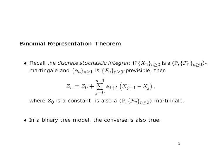
Binomial Representation Theorem Recall the discrete stochastic integral : if { X n } n 0 is a ( P , {F n } n 0 )- martingale and { n } n 1 is {F n } n 0 -previsible, then n 1 Z n = Z 0 + j +1 X j +1 X

SLIDE 1

Binomial Representation Theorem

Recall the discrete stochastic integral: if {Xn}n≥0 is a (P, {Fn}n≥0)-

martingale and {φn}n≥1 is {Fn}n≥0-previsible, then Zn = Z0 +

n−1

φj+1

Xj+1 − Xj
,

where Z0 is a constant, is also a (P, {Fn}n≥0)-martingale.

In a binary tree model, the converse is also true.

1

SLIDE 2

Suppose that the measure Q is such that the discounted price

process {˜ Sn} is a (Q, {Fn}n≥0)-martingale. If {˜ Vn} is any other (Q, {Fn}n≥0)-martingale, then there exists a (Q, {Fn}n≥0)- predictable process {φn}n≥1 such that ˜ Vn = ˜ V0 +

n−1

φj+1

Sj+1 − ˜ Sj

.
To prove this, we must show that

˜ Vi+1 − ˜ Vi = φi+1

Si+1 − ˜ Si

where φi+1 is Fi-measurable.

2

SLIDE 3

For a given node at t = iδt, write
˜

Si+1(u), ˜ Si+1(d)

for the

two possible values of ˜ Si+1, and

Vi+1(u), ˜ Vi+1(d)

for the

corresponding values of ˜ Vi+1.

We can solve

˜ Vi+1(u) − ˜ Vi = φi+1

Si+1(u) − ˜ Si

+ ki+1

and ˜ Vi+1(d) − ˜ Vi = φi+1

Si+1(d) − ˜ Si

+ ki+1

to get φi+1 = ˜ Vi+1(u) − ˜ Vi+1(d) ˜ Si+1(u) − ˜ Si+1(d).

3

SLIDE 4

Because
˜

Si+1(u), ˜ Si+1(d)

Vi+1(u), ˜ Vi+1(d)

are known

at time t = iδt, this φi+1 is Fi-measurable.

Also

ki+1 = ˜ Vi+1 − ˜ Vi − φi+1

Si+1 − ˜ Si

and because ki+1 is also Fi-measurable,

ki+1 = E

Vi+1 − ˜ Vi − φi+1

Si+1 − ˜ Si

Vi+1 − ˜ Vi

Fi
− φi+1E
˜

Si+1 − ˜ Si

because both {˜ Sn} and {˜ Vn} are (Q, {Fn}n≥0)-martingales.

That completes the proof.

4

SLIDE 5

Note that the tree did not need to be recombining, only

binary.

We did, however, tacitly assume that ˜

Si+1(u) = ˜ Si+1(d) at this node, and hence at all nodes.

Self-financing: we can build a dynamic portfolio of stock and

cash with discounted value {˜ Vn}, by holding φi+1 shares in [iδt, (i + 1)δt) and keeping the balance Vi − φi+1Si in cash.

5

SLIDE 6

Continuous Time Limit

Fix a time t > 0, and let δt = t/N; if N is large, and hence

δt is small, the binary tree should approximate a continuous time model.

At a node with stock price s, assume that the successor

nodes are s exp

νδt ± σ

√ δt

for a drift ν and volatility σ.
Suppose that under the market measure P, these are equally

likely.

6

SLIDE 7

Then the expected value at the next step, conditionally on

being at this node, is seνδt × 1 2

√ δt + e−σ √ δt

≈ s
1 +
ν + 1

2σ2

and the conditional variance is 1 4

seνδt2

eσ

√ δt − e−σ √ δt

2 ≈ s2σ2δt. whence the conditional standard deviation is sσ √ δt.

7

SLIDE 8

Suppose that by time t = Nδt, the price has moved up XN

times, and therefore down N − XN times.

Then

St = S0 exp

Nνδt + XNσ

√ δt − (N − XN) σ √ δt

= S0 exp
νt + σ

√ t

2XN − N

√ N

is binomial, so, by the Central Limit Theorem, ZN

△

= (2XN − N) / √ N is approximately standard normal for large N, so we can write this as St = S0 exp

νt + σ

√ tZN

where ZN is approximately N(0, 1).

8

SLIDE 9

So, under the market measure P, St is approximately log-

normally distributed.

Under the martingale measure Q, the probability of an up-

jump is p = erδt − eνδt−σ

√ δt

eνδt+σ

√ δt − eνδt−σ √ δt

≈ 1 2

 1 −

√ δt

 ν + 1

2σ2 − r

σ

    .

So XN is also binomial under Q, but with parameter p = 1

2.

9

SLIDE 10

Again using the CLT, under Q, (2XN − N) /

√ N is approxi- mately N

√ t

ν + 1

2σ2 − r

/σ, 1
.
So now we can write

St = S0 exp

r − 1

2σ2

t + σ

√ tZ∗

N

where Z∗

N △

= ZN + √ t

ν + 1

2σ2 − r

/σ is, now under Q, ap-

proximately N(0, 1).

Note that Z∗

N = ZN:

– ZN is approximately N(0, 1) under P; – Z∗

N is approximately N(0, 1) under Q.

10

SLIDE 11

Option pricing:

if a European option with maturity T has payoff C(ST), then its arbitrage-free price is EQ e−rTC(ST)

.
We would expect this to be approximately

EQ

e−rTC
S0 exp
r − 1

2σ2

T + σ

√ TZ∗

(although this follows from the convergence argument only

for bounded, continuous C(·)).

Here, under Q, Z∗ is approximately N(0, 1).

11