Bayes Nets (continued) [RN2] Section 14.4 [RN3] Section 14.4 CS - PDF document

Bayes Nets (continued) [RN2] Section 14.4 [RN3] Section 14.4 CS 486/686 University of Waterloo Lecture 9: Oct 9, 2012 Outline • Inference in Bayes Nets • Variable Elimination 2 CS486/686 Lecture Slides (c) 2012 C. Boutilier, P. Poupart & K. Larson 1

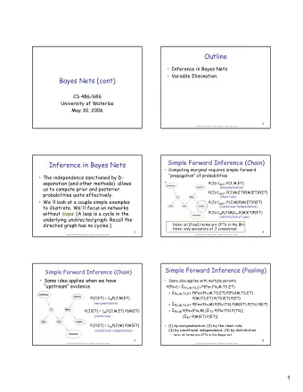
Inference in Bayes Nets • The independence sanctioned by D- separation (and other methods) allows us to compute prior and posterior probabilities quite effectively. • We'll look at a few simple examples to illustrate. We'll focus on networks without loops . (A loop is a cycle in the underlying undirected graph. Recall the directed graph has no cycles.) 3 CS486/686 Lecture Slides (c) 2012 C. Boutilier, P. Poupart & K. Larson Simple Forward Inference (Chain) • Computing marginal requires simple forward “propagation” of probabilities • P(J)=  M,ET P(J,M,ET) (marginalization) P(J)=  M,ET P(J|M,ET)P(M|ET)P(ET) (chain rule) P(J)=  M,ET P(J|M)P(M|ET)P(ET) (conditional independence) P(J)=  M P(J|M)  ET P(M|ET)P(ET) (distribution of sum) Note: all (final) terms are CPTs in the BN Note: only ancestors of J considered 4 CS486/686 Lecture Slides (c) 2012 C. Boutilier, P. Poupart & K. Larson 2

Simple Forward Inference (Chain) • Same idea applies when we have “upstream” evidence P(J|ET) =  M P(J,M|ET) (marginalisation) P(J|ET) =  M P(J|M,ET) P(M|ET) (chain rule) P(J|ET) =  M P(J|M) P(M|ET) (conditional independence) 5 CS486/686 Lecture Slides (c) 2012 C. Boutilier, P. Poupart & K. Larson Simple Forward Inference (Pooling) • Same idea applies with multiple parents P(Fev) = Σ Flu,M,TS,ET P(Fev,Flu,M,TS,ET) = Σ Flu,M,TS,ET P(Fev|Flu,M,TS,ET) P(Flu|M,TS,ET) P(M|TS,ET) P(TS|ET) P(ET) = Σ Flu,M,TS,ET P(Fev|Flu,M) P(Flu|TS) P(M|ET) P(TS) P(ET) = Σ Flu,M P(Fev|Flu,M) [ Σ TS P(Flu|TS) P(TS)] [ Σ ET P(M|ET) P(ET)] • (1) by marginalisation; (2) by the chain rule; (3) by conditional independence; (4) by distribution – note: all terms are CPTs in the Bayes net 6 CS486/686 Lecture Slides (c) 2012 C. Boutilier, P. Poupart & K. Larson 3

Simple Forward Inference (Pooling) • Same idea applies with evidence P(Fev|ts,~m) = Σ Flu P(Fev,Flu|ts,~m) = Σ Flu P(Fev |Flu,ts,~m) P(Flu|ts,~m) = Σ Flu P(Fev|Flu,~m) P(Flu|ts) 7 CS486/686 Lecture Slides (c) 2012 C. Boutilier, P. Poupart & K. Larson Simple Backward Inference • When evidence is downstream of query variable, we must reason “backwards.” This requires the use of Bayes rule: P(ET | j) = α P(j | ET) P(ET) = α Σ M P(j,M|ET) P(ET) = α Σ M P(j|M,ET) P(M|ET) P(ET) = α Σ M P(j|M) P(M|ET) P(ET) • First step is just Bayes rule – normalizing constant α is 1/P(j); but we needn’t compute it explicitly if we compute P(ET | j) for each value of ET: we just add up terms P(j | ET) P(ET) for all values of ET (they sum to P(j)) 8 CS486/686 Lecture Slides (c) 2012 C. Boutilier, P. Poupart & K. Larson 4

Backward Inference (Pooling) • Same ideas when several pieces of evidence lie “downstream” P(ET|j,fev) = α P(j,fev|ET) P(ET) = α Σ M,Fl,TS P(j,fev,M,Fl,TS|ET) P(ET) = α Σ M,Fl,TS P(j|fev,M,Fl,TS,ET) P(fev|M,Fl,TS,ET) P(M|Fl,TS,ET) P(Fl|TS,ET) P(TS|ET) P(ET) = α P(ET) Σ M P(j|M) P(M|ET) Σ Fl P(fev|M,Fl) Σ TS P(Fl|TS) P(TS) – Same steps as before; but now we compute prob of both pieces of evidence given hypothesis ET and combine them. Note: they are independent given M; but not given ET. 9 CS486/686 Lecture Slides (c) 2012 C. Boutilier, P. Poupart & K. Larson Variable Elimination • The intuitions in the above examples give us a simple inference algorithm for networks without loops: the polytree algorithm. • Instead we'll look at a more general algorithm that works for general BNs; but the polytree algorithm will be a special case. • The algorithm, variable elimination , simply applies the summing out rule repeatedly. – To keep computation simple, it exploits the independence in the network and the ability to distribute sums inward 10 CS486/686 Lecture Slides (c) 2012 C. Boutilier, P. Poupart & K. Larson 5

Factors • A function f(X 1 , X 2 ,…, X k ) is also called a factor . We can view this as a table of numbers, one for each instantiation of the variables X 1 , X 2 ,…, X k. – A tabular rep’n of a factor is exponential in k • Each CPT in a Bayes net is a factor: – e.g., Pr(C|A,B) is a function of three variables, A, B, C • Notation: f( X , Y ) denotes a factor over the variables X ∪ Y . (Here X , Y are sets of variables.) 11 CS486/686 Lecture Slides (c) 2012 C. Boutilier, P. Poupart & K. Larson The Product of Two Factors • Let f( X , Y ) & g( Y , Z ) be two factors with variables Y in common • The product of f and g, denoted h = f x g (or sometimes just h = fg), is defined: h( X , Y , Z ) = f( X , Y ) x g( Y , Z ) f(A,B) g(B,C) h(A,B,C) ab 0.9 bc 0.7 abc 0.63 ab~c 0.27 a~b 0.1 b~c 0.3 a~bc 0.08 a~b~c 0.02 ~ab 0.4 ~bc 0.8 ~abc 0.28 ~ab~c 0.12 ~a~b 0.6 ~b~c 0.2 ~a~bc 0.48 ~a~b~c 0.12 12 CS486/686 Lecture Slides (c) 2012 C. Boutilier, P. Poupart & K. Larson 6

Summing a Variable Out of a Factor • Let f(X, Y ) be a factor with variable X ( Y is a set) • We sum out variable X from f to produce a new factor h = Σ X f, which is defined: h( Y ) = Σ x ∊ Dom(X) f(x, Y ) f(A,B) h(B) ab 0.9 b 1.3 a~b 0.1 ~b 0.7 ~ab 0.4 ~a~b 0.6 13 CS486/686 Lecture Slides (c) 2012 C. Boutilier, P. Poupart & K. Larson Restricting a Factor • Let f(X, Y ) be a factor with variable X ( Y is a set) • We restrict factor f to X=x by setting X to the value x and “deleting”. Define h = f X=x as: h( Y ) = f(x, Y ) f(A,B) h(B) = f A=a ab 0.9 b 0.9 a~b 0.1 ~b 0.1 ~ab 0.4 ~a~b 0.6 14 CS486/686 Lecture Slides (c) 2012 C. Boutilier, P. Poupart & K. Larson 7

Variable Elimination: No Evidence • Computing prior probability of query var X can be seen as applying these operations on factors A B C f 2 (A,B) f 3 (B,C) f 1 (A) • P(C) = Σ A,B P(C|B) P(B|A) P(A) = Σ B P(C|B) Σ A P(B|A) P(A) = Σ B f 3 (B,C) Σ A f 2 (A,B) f 1 (A) = Σ B f 3 (B,C) f 4 (B) = f 5 (C) Define new factors: f 4 (B)= Σ A f 2 (A,B) f 1 (A) and f 5 (C)= Σ B f 3 (B,C) f 4 (B) 15 CS486/686 Lecture Slides (c) 2012 C. Boutilier, P. Poupart & K. Larson Variable Elimination: No Evidence • Here’s the example with some numbers A B C f 2 (A,B) f 3 (B,C) f 1 (A) f 1 (A) f 2 (A,B) f 3 (B,C) f 4 (B) f 5 (C) a 0.9 ab 0.9 bc 0.7 b 0.85 c 0.625 ~a 0.1 a~b 0.1 b~c 0.3 ~b 0.15 ~c 0.375 ~ab 0.4 ~bc 0.2 ~a~b 0.6 ~b~c 0.8 16 CS486/686 Lecture Slides (c) 2012 C. Boutilier, P. Poupart & K. Larson 8

VE: No Evidence (Example 2) A f 1 (A) C D f 4 (C,D) f 2 (B) B f 3 (A,B,C) P(D) = Σ A,B,C P(D|C) P(C|B,A) P(B) P(A) = Σ C P(D|C) Σ B P(B) Σ A P(C|B,A) P(A) = Σ C f 4 (C,D) Σ B f 2 (B) Σ A f 3 (A,B,C) f 1 (A) = Σ C f 4 (C,D) Σ B f 2 (B) f 5 (B,C) = Σ C f 4 (C,D) f 6 (C) = f 7 (D) Define new factors: f 5 (B,C), f 6 (C), f 7 (D), in the obvious way 17 CS486/686 Lecture Slides (c) 2012 C. Boutilier, P. Poupart & K. Larson Variable Elimination: One View • One way to think of variable elimination: – write out desired computation using the chain rule, exploiting the independence relations in the network – arrange the terms in a convenient fashion – distribute each sum (over each variable) in as far as it will go • i.e., the sum over variable X can be “pushed in” as far as the “first” factor mentioning X – apply operations “inside out”, repeatedly eliminating and creating new factors (note that each step/removal of a sum eliminates one variable) 18 CS486/686 Lecture Slides (c) 2012 C. Boutilier, P. Poupart & K. Larson 9

Variable Elimination Algorithm • Given query var Q, remaining vars Z . Let F be the set of factors corresponding to CPTs for {Q} ∪ Z . 1. Choose an elimination ordering Z 1 , …, Z n of variables in Z . 2. For each Z j -- in the order given -- eliminate Z j ∊ Z as follows: (a) Compute new factor g j = Σ Zj f 1 x f 2 x … x f k , where the f i are the factors in F that include Z j (b) Remove the factors f i (that mention Z j ) from F and add new factor g j to F 3. The remaining factors refer only to the query variable Q. Take their product and normalize to produce P(Q) 19 CS486/686 Lecture Slides (c) 2012 C. Boutilier, P. Poupart & K. Larson VE: Example 2 again Factors: f 1 (A) f 2 (B) A f 1 (A) f 3 (A,B,C) f 4 (C,D) C D Query: P(D)? f 4 (C,D) B f 2 (B) f 3 (A,B,C) Elim. Order: A, B, C Step 1: Add f 5 (B,C) = Σ A f 3 (A,B,C) f 1 (A) Remove: f 1 (A), f 3 (A,B,C) Step 2: Add f 6 (C)= Σ B f 2 (B) f 5 (B,C) Remove: f 2 (B) , f 5 (B,C) Step 3: Add f 7 (D) = Σ C f 4 (C,D) f 6 (C) Remove: f 4 (C,D), f 6 (C) Last factor f 7 (D) is (possibly unnormalized) probability P(D) 20 CS486/686 Lecture Slides (c) 2012 C. Boutilier, P. Poupart & K. Larson 10