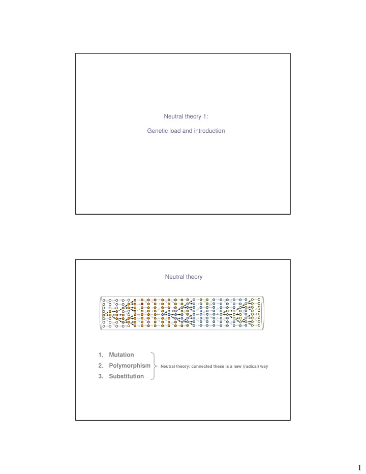

Neutral theory 1: Genetic load and introduction Neutral theory 1. Mutation 2. Polymorphism Neutral theory: connected these is a new (radical) way 3. Substitution 1
Neo-Darwinism 1. genetic variation arises at random via mutation and recombination 2. populations evolve by changes in allele frequencies 3. allele frequencies change by mutation, migration, drift and natural selection 4. most mutations are deleterious 5. most adaptive phenotypic effects are small so changes in phenotype are slow and gradual • some such changes can have large discrete effects 6. diversification occurs by speciation • usually a gradual process • usually by geographic isolation microevolution ⇒ macroevolution 7. Neo-Darwinism Classical school Balance school • Most new mutations are deleterious • Most new mutations are deleterious • Natural selection is of central importance • Natural selection is of central importance •Polymorphism is a function of selection •Polymorphism is a function of selection • Polymorphism is very rare • Polymorphism is common • Positive Darwinian selection and •Balancing selection is comparable to balancing selection are rare with respect to purifying selection in micro-evolution purifying selection in micro-evolution • Genetic variation connected to • Too much “genetic load” for genetic morphological variation. variation to connect with morph. variation • Prediction : most populations will be • Prediction : most populations will be heterozygous at most loci homozygous at most loci 2
“ It is altogether unlikely that two genes would have identical selective values under all the conditions under which they may coexist in a population. … cases of neutral polymorphism do not exist … it appears probable that random fixation is of negligible evolutionary importance ” ⎯ Ernst Mayr Neo-Darwinism 1930’s: ⎯ no way to test the predictions of different schools ⎯ arguments centered on mathematical models 1950’s and 1960’s: ⎯ protein sequencing ( slow and painful ) ⎯ protein gel electrophoresis ( fast and cheap ) 3
Protein electrophoresis: big changes in the 1960’s (A) Diagram of a protein gel electrophoresis apparatus, and (B) a photograph of a “stained” protein gel, the blue “blotches” are the proteins, their position indicates how far they migrated in the electric field. A B Protein electrophoresis: the results are in … Lewontin and Hubby (1966): Harris (1966): • 5 natural populations of Drosophila • Humans • 18 loci • 71 loci • 30% of loci (27 over the 5 popn.s) • 28% (20) were polymorphic were polymorphic • Human heterozygosity: 7% (2-53%) • Fruitfly heterozygosity: 11% Balance school: predictions correct ! Classical school: predictions wrong (But, what about load!) Lewontin and Hubby (1966) suggested that some of the polymorphism must be neutral 4
Genetic load Genetic load: the extent to which the fitness of an individual is below the optimum for the population as a whole due to the deleterious alleles that the individual carries in its genome. W = average fitness Genetic load (L) = 1 - W Genetic load: an example Two alleles ( A and a) with frequencies p = q = 0.5: Survival to reproduce: AA = 40% Aa = 50% aa = 30% The relative fitness values are: AA = 0.8 Aa = 1 aa = 0.6 The mean fitness of the population = 0.25(0.8) + 0.5(1) + 0.25(0.6) = 0.85 The load of this population (L) = 1 – 0.85 = 0.15 [ Note that if every member of the population had the same genotype the average fitnes would equal 1 and the load on the population would be zero.] Selective death (or genetic death): the chance that an individual will die without reproducing as a consequence of natural selection. [ e.g.,15% of offspring in above ] 5
Genetic load: the cost of selection [ or “ Haldane’s dilemma ”] Genetic load has implications for the long term fate of a population. Haldane: the total load tolerated by a population is bounded by its excess reproductive capacity. Suppose L = 0.1 Haldane’s “Cost of selection” Load = 10% population reduction Total size = 500 individuals (1957) Reproductive size: 450 Cost of selection (C) = L/ = 0.1/0.9 = 0.111 W propotion that die due to selection ∑ ∑ = = L C proportion that survive W C x N = 50 extra individuals per generation 1 4 4 4 4 4 4 4 4 2 4 4 4 4 4 4 4 4 3 over all generation s it takes to fix the allele Total generation to fix allele = 100 Population 1: Population 2: Reproductive excess = 0 Reproductive excess = 0.1 Generation = 100 Generation = 53 - fixed beneficial allele - Extinction: CxN=499.1 Population declines: - CxN = 334.6 Genetic death > reproductive excess - survival: N =165.4 Genetic load: sources 1. Mutational load 2. Substitutional load [Haldane’s load] 3. Segregational load 6
Genetic load: mutational Let’s assume: (i) new mutations are deleterious alleles, and (ii) recessive. Remember the approximation of the equilibrium frequency of deleterious alleles [See population genetics, Topic 5 for a review]: q = ( µ /s) 1/2 Remember that population load is: L = 1 - W And remember that the average fitness under these assumptions was: = 1 – sq 2 W We can make substitutions: W L = 1 - L = 1 – (1 – sq 2 ) L = 1 – (1 – s( µ /s)) L = 1 – (1 – µ ) L = µ It is interesting that we estimate that the load is equal to the mutation rate. Because it suggests that the load is approximately independent of the reduction in fitness caused by the mutant ( s ). Genetic load: mutational Mutational load is minor: 1. Equilibrium yields a polymorphism involving an allele that is very rare in the population 2. The load is trivial 7
Genetic load: substitutional Deleterious recessive Genotype AA Aa aa Frequency p 0 2 2 p 0 q 0 q 0 2 w model 1 1 1 - s 1 1 0.66 w Haldane’s “cost of selection” is associated with fixation of an allele under a model such as the one above. Haldane assumed this type of lead to estimate that the maximum rate of fixation of mutations in humans could not exceed 1 in 300 generations Genetic load: segregational The model Genotype AA Aa aa Frequency p 0 2 2 p 0 q 0 q 0 2 1 – s 1 1 1 – s 2 w Segregational load is a big problem for the balance school: Well known examples exist; Haemoglobin, MHC locus, etc. Balance school would extend this to most polymorphic loci in the genome. Let’s see if this will work. Humans: 30% of loci are polymorphic (from Harris 1966) 30,000 genes (from recent genome projects), so 9000 are polymorphic Let’s assume a very small load on average: L = 0.001 Let’s assume that only half are under balancing selection (4500) [remember the balance school predicted a majority would be under balancing selection] Fitness of an individual locus = 0.999 Fitness over whole genome = 0.999 4500 = 0.011 Load = 1- 0.011 = 0.090 [That is huge!!!] Cost = 0.989/0.011 = 89 [Do you know of any humans with families that big?] 8
Genetic load: other 1. Recombinational load 2. Incompatibility load 3. Lag load Note: all load arguments tend to be based on overly-simplistic models. Neutral theory of molecular evolution Motoo Kimura: • troubled by cost Haldane’s dilemma: • 1 substitution every 300 generations • troubled by Zukerkandl and Pauling’s (1965) molecular clock: • 1 substitution every 2 years Published a model of neutral evolution in 1968 Jack King and Thomas Jukes: Independently arrived at same conclusion as Kimura Published (1969) under the provocative title “Non-Darwinian evolution” I cannot over emphasize how radical this idea was at that time. 9
Neutral theory of molecular evolution: elegant simplicity k = rate of nucleotide substitution at a site per generation [year] k = new mutations × probability of fixation Number of new mutations = µ × 2 N e 1 Probability of fixation = 2 N e Hence, the neutral rate is: = µ × 2 N e × k 1/2 N e = µ k Neutral theory of molecular evolution Neutral theory: the rate of evolution is independent of effective population size • mutations-drift equilibrium • assumes (i) neutrality and (ii) constant mutation rate • polymorphism is simply a phase of evolution ( mutation, polymorphism and substitution are not separate processes ) Evolution by natural selection: k = µ × 4 N e × s • rate depends on mutation rate and population size and intensity of selection 10
Remember the genetic drift lecture… If we run this simulation long enough it will go to fixation of loss; it just takes much longer • rate to fixation [under drift] slows with increasing in N e • ultimate fate is fixation or loss • Larger N e yield larger residence time of a polymorphism in a population The average time to fixation is 4 N e generations Time to fixation ( t ) of new alleles in populations with different effective sizes. Note that most new mutations are lost from the population due to drift and those mutations are NOT shown. The time to fixation (as an average) is longer in populations with large size. N e = small 1 Allele frequency 0 t N e = large 1 Allele frequency 0 t A slice in time for each population is shown by a dotted vertical line ( ). Note that at such a slice in time the population with larger effective size is more polymorphic as compared with the smaller population. 11
Recommend
More recommend