Asynchronous DP, Real-Time DP and Intro to RL Lecturer: Daniel Russo - PDF document
Lecture number - Oct 3 B9140 Dynamic Programming & Reinforcement Learning Asynchronous DP, Real-Time DP and Intro to RL Lecturer: Daniel Russo Scribe: Kejia Shi, Yexin Wu Todays lecture looks at the following topic: Classical DP:
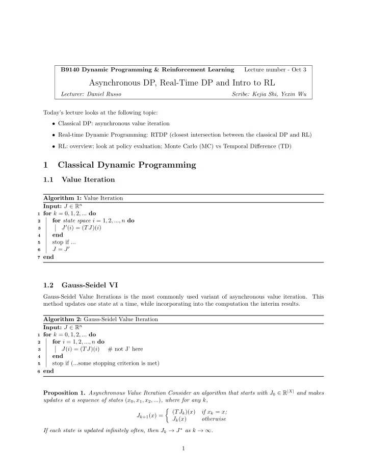
Lecture number - Oct 3 B9140 Dynamic Programming & Reinforcement Learning Asynchronous DP, Real-Time DP and Intro to RL Lecturer: Daniel Russo Scribe: Kejia Shi, Yexin Wu Today’s lecture looks at the following topic: • Classical DP: asynchronous value iteration • Real-time Dynamic Programming: RTDP (closest intersection between the classical DP and RL) • RL: overview; look at policy evaluation; Monte Carlo (MC) vs Temporal Difference (TD) 1 Classical Dynamic Programming 1.1 Value Iteration Algorithm 1: Value Iteration Input: J ∈ R n 1 for k = 0 , 1 , 2 , ... do for state space i = 1 , 2 , ..., n do 2 J ′ ( i ) = ( TJ )( i ) 3 end 4 stop if ... 5 J = J ′ 6 7 end 1.2 Gauss-Seidel VI Gauss-Seidel Value Iterations is the most commonly used variant of asynchronous value iteration. This method updates one state at a time, while incorporating into the computation the interim results. Algorithm 2: Gauss-Seidel Value Iteration Input: J ∈ R n 1 for k = 0 , 1 , 2 , ... do for i = 1 , 2 , ..., n do 2 J ( i ) = ( TJ )( i ) # not J’ here 3 end 4 stop if (...some stopping criterion is met) 5 6 end Proposition 1. Asynchronous Value Iteration Consider an algorithm that starts with J 0 ∈ R | X | and makes updates at a sequence of states ( x 0 , x 1 , x 2 , ... ) , where for any k , � ( TJ k )( x ) if x k = x ; J k +1 ( x ) = J k ( x ) otherwise If each state is updated infinitely often, then J k → J ∗ as k → ∞ . 1
Proof. Case 1: If J 0 � TJ 0 , then we have J 0 � TJ 0 � T 2 J 0 � ... � T k J 0 � ... � J ∗ . We also have J 0 � TJ 0 = J 1 , since our assumption. We change only one state of them and get it bigger with other states untouched. By monotonicity, we have J 1 � TJ 0 � TJ 1 . Repeating this we have J 2 � J 1 and J 2 � TJ 2 . Inductively, J 0 � J 1 � J 2 � ... � J k and J k � TJ k , which implies J k � J ∗ . Let J ∞ = lim k →∞ J k . Certainly we have J ∞ = TJ ∞ . (run forever, get arbitrarily close) Note: J k +1 ( x k ) − J k ( x k ) = TJ k ( x k ) − J k ( x k ): RHS: Bellman gap; LFS: goes to 0 when k → ∞ . Case 2: If J 0 � TJ 0 , then similar to case 1, just flip everything around. Case 3: For any J 0 , take δ > 0, e = (1 , 1 , ..., 1), we have J − ≡ J ∗ − δe � J 0 � J ∗ + δe ≡ J + . k be the output of asynchronous value iteration applied to J − and J + . Let J − k , J + k . One can show that J − � TJ − , J + � TJ + . Monotonicity gives us J − k � J k � J + So J + → J ∗ and J − → J ∗ , which means J k → J ∗ . Note: Another way to prove is through contractions. Here we use monotonicity. Intuitively, everywhere we update, it’s a right direction with its momentum maintained. Why we do this? • Distributed computation: most DPs have too many states, the real case is that you can’t update states in a line. Some are slower than the others. (Communication delays, see textbook Chap 2.6) • Form the basis of learning from interaction: most RL algos look at TJ k at x k . 2 Real-Time Dynamic Programming This is a variant of asynchronous value iteration where states are sampled by an agent that, at all times, makes decisions greedily under her current guess of the value function. The following proposition gives a first Algorithm 3: Real-Time Dynamic Programming Input: J 0 1 for k = 0 , 1 , 2 , ... do observe x k the current state 2 play u k = arg min u g ( x, u ) + γ Σ x ′ P ( x, u, x ′ ) J k ( x ′ ) 3 update J k +1 ( x ) = TJ k ( x ) if x = x k ; otherwise J k +1 ( x ) = J k ( x ) 4 5 end convergence result for RTDP. For details see [BBS95]. Note that unlike the previous case, this proposition does not require that every state is visited infinitely often. 2
Proposition 2. Under RTDP, J k converges to some vector J ∞ , J ∞ ( x ) = TJ ∞ ( x ) at all x visited i.o. Note: This proposition is unsatisfying since it does not imply convergence to J ∗ . To guarantee convergence to J ∗ using the previous result, we would generally need to ensure each state is updated infinitely often. However, it’s not clear the goal should be to find J ∗ , at all. Instead, it may be sufficient that eventually the action’s chosen by the agent are optimal. Fix 1: We may add randomness to action selection in an effort to ensure that every state is visited infinitely often. If each state is reachable from any other state, this will work, and is enough to ensure asymptotic convergence of J k to J ∗ . However, it may take an exceptionally long time to reach visit certain states. One reason is that random exploration can be very inefficient, and may take such a strategy time exponential in the size of the state space to reach a state that could be reached efficiently under a particular policy. But it may also be the case that some states are almost impossible to reach under any policy. It seems that these states are essentially irrelevant to minimizing discounted costs. Fix 2: Start optimistic. Assume J 0 � TJ 0 . This can be ensure by picking a J 0 that has very small values (e.g. if expected costs are non-negative, it suffices to take J 0 = 0) From the above we have J 0 � J 1 � J 2 � ... and so on. (This means we always believe expected costs are lower than is possible, and updates always consist of raising our expectations about expected costs.) Proposition 3. If J 0 � TJ 0 , there exists a (random) time K after which all actions are optimal. That is u k = µ ∗ ( x k ) for any K > k . Note J k � J k +1 � ... � J ∗ , so J k → J ∞ . (bounded monotone sequences converge.) This implies the policy also converges, µ k → µ ∞ : The following argument holds for any sample path, (omitting a set of measure zero). • Let V be the set of states visited i.o. (this exists and is nonempty for any sample path). • The agent’s eventual policy µ ∞ must have zero probability of leaving V . (Precisely, P ( x, µ ∞ ( x ) , x ′ ) = 0 for all x ′ ∈ V c ). Otherwise, with probability 1 the agent would eventually leave V . – It is as if the agent plays on a sub-MDP where all sates in V c have been deleted, and all actions that might reach V c are deleted. – As a result, the estimates J ∞ ( x ) are accurate for all x ∈ V . That is J ∞ ( x ) = J µ ∞ ( x ), the agent’s true expected cost-to-go under the current policy. • How do we conclude the actions chosen by µ ∞ on V are optimal? – Consider some action u � = µ ∞ ( x ). Since u is not chosen, it must be that � � P ( x, µ ∞ ∞ , x ′ ) J ∞ ( x ′ ) ≤ g ( x, u ) + γ P ( x, u, x ′ ) J ∞ ( x ′ ) g ( x, µ ∞ ( x )) + γ x ′ ∈ X x ′ ∈ X But by he discussion above, the left hand side equals J µ ( x ), and so the true cost of following µ is less than estimated cost of playing u with cost-to-go under J ∞ . – From here, the key is that J ∞ ( x ) ≤ J ∗ ( x ) for all x ∈ V c . The agent may not have an accurate estimate of the value function, but is optimistic , in sense that she underestimates costs at V c . – In particular, for x ∈ V , and u � = µ ∞ ( x ) � � P ( x, u, x ′ ) J ∞ ( x ′ ) ≤ g ( x, u ) + γ P ( x, u, x ′ ) J ∗ ( x ′ ) g ( x, u ) + γ x ′ ∈ X x ′ ∈ X Therefore, the cost of playing u with cost-to-go estimate J ∞ underestimates the real cost from playing u , even if actions thereafter are chosen optimally. If J µ ( x ) is below this under-estimate, u cannot be optimal. 3
Recommend
More recommend
Explore More Topics
Stay informed with curated content and fresh updates.
