Optimal Control and Dynamic Programming 4SC000 Q2 2017-2018 Duarte - PowerPoint PPT Presentation
Optimal Control and Dynamic Programming 4SC000 Q2 2017-2018 Duarte Antunes Part I Discrete optimization problems Outline Dynamic programming formalism Stochastic dynamic programming Applications Recap c 1 c 0 n 1 n 1 1 n 0 2 c h
Optimal Control and Dynamic Programming 4SC000 Q2 2017-2018 Duarte Antunes
Part I Discrete optimization problems
Outline • Dynamic programming formalism • Stochastic dynamic programming • Applications
Recap c 1 c 0 n 1 n 1 1 n 0 2 c h − 1 c 0 n h − 1 1 c h n h n 0 n 0 1 1 − n h n h c 1 c 0 23 22 c h − 1 c 1 c 0 22 22 21 2 2 2 c h − 1 c 0 c 1 12 21 21 c h 1 c h − 1 c 0 c 1 11 11 11 1 1 1 1 Stage 0 Stage 1 Stage h − 1 Stage h • Discrete optimization problem specified by a transition diagram. • Several applications. 1
Recap The dynamic programming algorithm provides a policy from which an optimal path can be obtained. Policies are crucial to cope with disturbances. 4 1 3 5 3 3 2 0 1 1 2 1 3 0 4 1 2 2 4 4 2 5 5 1 4 0 1 3 7 1 9 4 4 5 1 3 3 2 1 1 1 3 3 4 0 1 4 2 2 1 5 4 4 3 1 1 2
Equivalent formulation of discrete optimization problems • Dynamic model x k +1 = f k ( x k , u k ) , k ∈ { 0 , . . . , h − 1 } . h − 1 X g k ( x k , u k ) + g h ( x h ) . • Cost k =0 c 1 c 0 n 1 n 1 1 n 0 2 c h − 1 c 0 n h − 1 1 c h n h n 0 n 0 1 1 − n h c 1 c 0 23 22 n h c h − 1 c 1 c 0 22 22 21 2 2 2 c 0 c h − 1 c 1 12 c h 21 21 1 c h − 1 c 0 c 1 11 11 11 1 1 1 1 x h ∈ { 1 , . . . , n h } State x 1 ∈ { 1 , . . . , n 1 } x 0 ∈ { 1 , . . . , n 0 } Action u 0 ∈ { 1 , . . . , m 0 ,x 0 } u 1 ∈ { 1 , . . . , m 1 ,x 1 } Cost g 0 ( x 0 , u 0 ) = c 0 g h ( x h ) = c h g 1 ( x 1 , u 1 ) = c 1 3 x h x 0 ,u 0 x 1 ,u 1
Dynamic programming equations Dynamic programming algorithm in the new formalist Start with for every and for each decision stage, starting J h ( i ) = g h ( i ) i ∈ X k from the last and moving backwards, compute and from k ∈ { h − 1 , h − 2 , . . . , 0 } J k µ k J k ( i ) = j ∈ U k ( i ) g k ( i, j ) + J k +1 ( f k ( i, j )) min DP equation and µ k ( i ) = j, where is the minimizer in the dynamic programming (DP) equation, i.e., j J k ( i ) = g k ( i, µ k ( i )) + J k +1 ( f k ( i, µ k ( i ))) and . Then is an optimal policy. { µ 0 , . . . , µ h − 1 } U k ( i ) := { 1 , . . . , m k,i } 4
Remarks • The DP equation expresses the balance each optimal decision must meet between immediate and future cost J k ( x k ) = min g ( x k , u k ) + J k +1 ( f ( x k , u k )) u k ∈ U k ( x k ) | {z } | {z } immediate or stage cost future cost • This is just a more formal way of writing what we have already seen. • We shall use the same notation for stage-decision problems. • There we shall formally prove that the dynamic programming algorithm provides the optimal policy. The proof also applies to discrete optimization problems. 5
Example Move a robot from an initial stage to a final stage in minimum time 0 h initial stage final stage 0 h • If the robot is not stuck in an obstacle or in a wall it can go up, straight or down. Otherwise, there is only one option (see figs). It takes I time unit to move horizontally from stage to stage and to move diagonally. time units are √ i + 1 i 2 c paid every time an obstacle or a wall is hit. √ 2 √ √ √ 1 + c 1 2 + c 2 + c 2 lower wall obstacle up straight down upper wall 6
Modeling This problem can be written in the DP framework for a transition diagram obtained from the rules of the problem √ √ 2 + c 2 + c √ 2 √ 2 1 1 √ √ 2 2 √ 2 1 1 + c 7
DP equation n 1 final stage h initial stage 0 J h ( i ) = 0 i ∈ { 1 , . . . , n } For : k ∈ { h − 1 , h − 2 , . . . , 1 , 0 } √ J k (1) = 2 + c + J k +1 (2) √ J k ( n ) = 2 + c + J k +1 ( n − 1) √ √ not an obstacle node J k ( i ) = min { 1 + J k +1 ( i ) , 2 + J k +1 ( i + 1) , 2 + J k +1 ( i − 1) } obstacle node J k ( i ) = 1 + c + J k +1 ( i ) i ∈ { 2 , . . . , n − 1 } 8
Numerical Example √ J k ( n ) = 2 + c + J k +1 ( n − 1) J h ( i ) = 0 17.4116.4115.4114.4113.4112.4111.4110.419.41 8.41 7.41 6.41 5.41 0.00 13.0012.0011.0010.009.00 8.00 7.00 6.00 5.00 4.00 3.00 2.00 1.00 0.00 13.4112.4111.4110.419.41 8.41 11.416.41 5.41 8.41 3.41 6.00 1.00 0.00 13.8312.8311.8310.839.83 9.24 11.416.41 5.41 4.41 3.41 6.00 1.00 0.00 13.8312.8311.8310.839.83 8.83 7.83 6.83 5.83 8.00 3.00 2.00 1.00 0.00 14.2413.2412.2411.2410.249.24 12.247.24 9.41 8.41 3.41 6.00 1.00 0.00 13.8312.8311.8310.839.83 12.8311.836.83 9.41 8.41 3.41 6.00 1.00 0.00 13.4112.4111.4110.419.41 8.41 11.416.41 5.41 8.00 3.00 2.00 1.00 0.00 13.0012.0011.0010.009.00 8.00 7.00 6.00 5.00 4.00 3.00 2.00 1.00 0.00 13.0012.0011.0010.009.00 8.00 7.00 6.00 5.00 4.00 3.00 2.00 1.00 0.00 : 13.0012.0011.0010.009.00 8.00 7.00 6.00 5.00 4.00 3.00 2.00 1.00 0.00 13.0012.0011.0010.009.00 8.00 7.00 6.00 5.00 4.00 3.00 2.00 1.00 0.00 17.4116.4115.4114.4113.4112.4111.4110.419.41 8.41 7.41 6.41 5.41 0.00 √ J k (1) = 2 + c + J k +1 (2) c = 4 √ √ not an obstacle node J k ( i ) = min { 1 + J k +1 ( i ) , 2 + J k +1 ( i + 1) , 2 + J k +1 ( i − 1) } obstacle node J k ( i ) = 1 + c + J k +1 ( i ) 9
Outline • Dynamic programming formalism • Stochastic dynamic programming • Applications
Discussion • We can use the policy provided by the dynamic programming algorithm assuming no disturbances to cope with disturbances. • Is this procedure optimal in any sense? In general, no. • In fact, as we show next, in the presence of disturbances it may not even be possible to define optimal decisions, since these would depend on future realizations of disturbances. 10
Example 17.4116.4115.4114.4113.4112.4111.4110.419.41 8.41 7.41 6.41 5.41 0.00 13.0012.0011.0010.009.00 8.00 7.00 6.00 5.00 4.00 3.00 2.00 1.00 0.00 Consider that at position A there might 13.4112.4111.4110.419.41 8.41 11.416.41 5.41 8.41 3.41 6.00 1.00 0.00 be a disturbance making the robot move 13.8312.8311.8310.839.83 9.24 11.416.41 5.41 4.41 3.41 6.00 1.00 0.00 13.8312.8311.8310.839.83 8.83 7.83 6.83 5.83 8.00 3.00 2.00 1.00 0.00 down one extra position A 14.2413.2412.2411.2410.249.24 12.247.24 9.41 8.41 3.41 6.00 1.00 0.00 13.8312.8311.8310.839.83 12.8311.836.83 9.41 8.41 3.41 6.00 1.00 0.00 13.4112.4111.4110.419.41 8.41 11.416.41 5.41 8.00 3.00 2.00 1.00 0.00 13.0012.0011.0010.009.00 8.00 7.00 6.00 5.00 4.00 3.00 2.00 1.00 0.00 13.0012.0011.0010.009.00 8.00 7.00 6.00 5.00 4.00 3.00 2.00 1.00 0.00 13.0012.0011.0010.009.00 8.00 7.00 6.00 5.00 4.00 3.00 2.00 1.00 0.00 13.0012.0011.0010.009.00 8.00 7.00 6.00 5.00 4.00 3.00 2.00 1.00 0.00 17.4116.4115.4114.4113.4112.4111.4110.419.41 8.41 7.41 6.41 5.41 0.00 Possible outcomes (no disturbance/ disturbance) √ 2 √ 1 2 1 √ 5 √ 2 1 down up straight Decisions 11
Example no disturbance disturbance √ decision: ‘up’ 11 . 4 + 2 7 . 83 + 1 √ decision:‘straight’ 7 . 83 + 1 12 . 2 + 2 √ decision:‘down’ √ 11 . 8 + 5 12 . 2 + 2 cost-to-go at position A If we knew the future disturbance value, we would pick ‘up’ if ‘disturbance’, ‘straight’ if ‘no disturbance’. Thus, if we assume nothing about the disturbances there is no optimal decision at position A. 12
Assumptions on disturbances There are two assumptions that make optimal decisions well-defined • Stochastic disturbances. If we have a stochastic characterization of disturbances we can define optimal policies as the ones that minimize the expected cost. The dynamic programming framework can be extended to provide this policy. • Worst-case disturbances. Optimal control problems with worst-case disturbances can be tackled in the framework of game theory and will not be addressed in the course. 13
Example: stochastic disturbances For the toy robot problem consider the stochastic characterization: Prob[disturbance] = 0 . 2 Prob[no disturbance] = 0 . 8 no disturbance disturbance Expected cost decision: ‘up’ √ √ (11 . 4 + 2)0 . 8 + (7 . 83 + 1)0 . 2 = 12 . 0174 11 . 4 + 2 7 . 83 + 1 decision:‘straight’ √ √ (7 . 83 + 1)0 . 8 + (12 . 2 + 2)0 . 2 = 9 . 79 12 . 2 + 2 7 . 83 + 1 √ √ decision:‘down’ √ (12 . 2 + 2)0 . 8 + (11 . 8 + 5)0 . 2 = 13 . 69 √ 11 . 8 + 5 12 . 2 + 2 cost-to-go at position A Optimal decision is now well-defined: pick ‘straight’ . 14
Example: worst-case disturbances no disturbance disturbance Worst-case cost decision: ‘up’ √ √ 11 . 4 + 2 7 . 83 + 1 11 . 4 + 2 √ √ decision:‘straight’ 12 . 2 + 2 12 . 2 + 2 7 . 83 + 1 √ √ √ decision:‘down’ 11 . 8 + 5 11 . 8 + 5 12 . 2 + 2 cost-to-go at position A Optimal decision is now well-defined: pick ‘up’. Safe policy (at least we get ). √ 11 . 4 + 2 15
Stochastic formulation: Markov decision processes The dynamic model and the cost take now the form x k +1 = f k ( x k , u k , w k ) h − 1 X g k ( x k , u k , w k ) + g h ( x h ) , k =0 where the state and input live in the same finite spaces defined before (slide 3), and disturbances belong to a finite set w k ∈ W k ( i, j ) := { 1 , . . . , ω i,j,k } when and are characterised by x k = i, u k = j p k,i,j := Prob[ w k = ` | x k = i, u k = j ] , ` ∈ W k ( i, j ) . ` Note that both the state and cost are now random variables. 16
Recommend
More recommend
Explore More Topics
Stay informed with curated content and fresh updates.
